Introduction

Some of the factors that bear on important decisions we make are linked. For example, we might not know how much demand there will be for an online service, but we know that if it is at the high end of our expectations then the load on the servers and networks used to deliver it are likely to be high too. Modelling such relationships in quantitative risk analysis must be done with great care. Ignoring them can result in outcomes that are wrong, sometimes significantly so, and that have the potential to mislead the users of an analysis.

This tutorial note examines the topic of correlation, the statistical term for the degree to which the variation in one factor will be related to variation in one or more other factors. It suggests some practical ways to incorporate correlations, or the relationships that give rise to them, in quantitative risk analysis models.

Foundations: quantitative models

Quantitative models of the kind in which we are interested use data from the past or the present (the inputs) to analyse what has been happening and to make predictions about the future (the outputs). In most circumstances the purpose of modelling is to provide insight to support better decisions.

Often the inputs are numbers. They might be:

• Physical constants (e.g. the expansion coefficient of steel)
• Prescribed constants (e.g. regulatory or policy thresholds)
• Data or estimates relating to external factors that demonstrate inherent variability (e.g. rainfall)
• Data or estimates relating to factors that may be difficult to predict precisely (e.g. market prices)
• Numbers associated with decisions and over which we may be able to exercise a degree of control.

The quantitative models combine the input numbers in some way – in our work, we often use equations and formulae in spreadsheets – to calculate the outputs. This is a straightforward process (although the calculations may not be!), so long as the inputs are numbers.

If the inputs are uncertain values rather than fixed numbers, then the calculations and the modelling process that supports them must work with this uncertainty.

For example, where there is uncertainty about something important, then a simple number may imply more precision and predictability than can be justified, or the decision maker may want to explore the underlying uncertainty in more detail. In these circumstances it is usually necessary to represent the uncertainty by a range or a distribution of values rather than a single number, and the model outputs will themselves be distributions, or numbers derived from distributions.

Spreadsheets alone are rarely suitable for the calculations that convert inputs in the form of distributions into outputs that are also distributions. Monte Carlo simulation is the technique most often used to represent uncertain values and evaluate the models that combine them, implemented in Excel with simulation add-ins such as @RISK (from Palisade) or ModelRisk (from Vose Software). In a Monte Carlo simulation, the calculations in the quantitative model are repeated many times, with input values that are sampled from their associated distributions in each iteration, and the calculated values are used to construct distributions of the model outputs. The process can be thought of as a series of what-if analyses that test the implications of all the possible combinations of inputs we can envisage, subject to the likelihood of those input values arising.

Spreadsheet tools that can work with uncertain values are not all that is required, though. Model structures must also be adjusted to make realistic calculations with distributions and, in particular, to take account of correlation.

Correlation and why it matters

What is correlation?

Entities such as datasets or probability distributions of forecast values of variables are said to be correlated if there is a mutual relationship or association between them that can be observed, anticipated in forecasts or modelled in real data. Such a relationship might indicate that one quantity is driving or causing change in the other. Alternatively, it might mean that a third factor, not in represented explicitly the model, is driving both of them.

The extent or strength of the relationship is measured by the correlation coefficient R, a value that lies between -1 (a perfect inverse relationship where high values of one factor will be associated with low values of the other) and +1 (a perfect direct relationship where high values of one factor will be associated with high values of the other). A value of zero means that there is no correlation between the datasets or distributions.

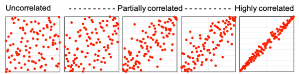
Figure 1 shows some examples.

• On the left, there is little obvious relationship between the data sets on the horizontal and vertical axes. These are uncorrelated, or independent, and the correlation coefficient R = 0.
• On the right, there is a strong direct link between the data sets. These are highly correlated, and R is close to 1.
• The intermediate diagrams show the relationships between data sets as R increases from 0 to 1.
• A strong negative correlation, with R close to -1, would show closely-linked points like the right-hand diagram, but with the points running in the other direction from the top-left to the bottom-right corner.

Why does correlation matter in quantitative risk analysis?

Appropriate treatment of correlations is essential in quantitative risk analysis. When each distribution is sampled for a Monte Carlo simulation, it is important that correlation is taken into account so that relationships expected in reality between inputs, like those in Figure 1, are reflected in the simulation output. If two values will actually lie at the high end of their separate ranges, or both lie at the low end of their ranges, or both fall in the middle, it is important that a model does not allow for a high value of one and a low value of the other to arise at the same time.

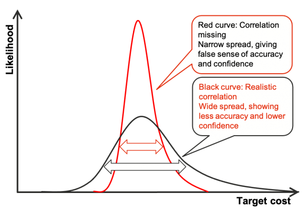
Figure 2 is an example of the output of a simulation of the cost of a project, illustrating why determining whether correlation exists (or not) is so important in quantitative risk analysis modelling.

• In the absence of correlation, when variables are independent of one another, a high value of one variable may balance out a low value of another, and therefore the sum of a group of uncertain variables will have the narrowest spread if they are all independent or if correlation is ignored (the red curve).
• Conversely, the greater the level of dependence or positive correlation, the greater the spread, because when correlation is present high values will tend to arise together, and so will low values, making extreme outcomes more likely to occur (the black curve).
• Because positive correlations between inputs have the effect of widening the output distributions from a simulation, from the red curve to the black curve, ignoring correlations when they exist in practice can result in large errors in the outputs, by making them appear more predictable than they really are.

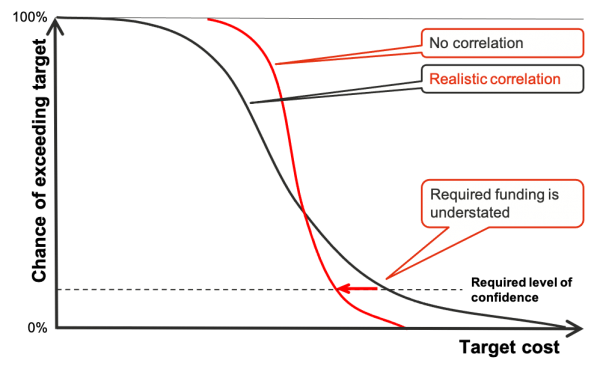
Correlation has a material effect at the extremities of the outcome distribution. For example, a director might want to set a project authorisation budget value at which there is only one chance in ten of an overrun, i.e. a budget in which she had 90% confidence. Using the cumulative form of the distributions, Figure 3 shows how a large error might arise in the budgeting process if correlation is present but not included appropriately in the model. (The cumulative distribution forms in Figure 3 are often easier to use than the density forms in Figure 2 if percentile values are important for making decisions.)

Modelling correlation

Direct estimates of correlation

Most simulation tools, such as @RISK and ModelRisk, allow correlation coefficients to be included explicitly in quantitative models. That sounds like a simple solution to modelling correlation, but it is still necessary to determine the appropriate coefficients.

If there is reliable historical data, and if it is reasonable to assume the future will be like the past, then calculating correlation coefficients is a simple mathematical exercise. If suitable data is available, then use it.

However, if there is little reliable data, then correlation factors can be estimated, although estimating correlation levels subjectively is not possible with any degree of reliability. One approach is to use scatter plots to visually represent different degrees of correlation (like Figure 1) and then select the one that ‘looks right’, but in fact such scatter plots vary considerably depending on factors such as whether the distributions that are being correlated are all the same shape, and what those shapes are. In addition, when using this approach, it can be very difficult to justify the choice of correlation coefficient to senior managers who must make important decisions based on the model outputs; if they don’t understand or have faith in the process and the inputs, they are unlikely to accept the results and the modelling effort has been wasted.

Estimating bounds on the effects of correlation

An alternative to estimating individual correlation coefficients is to estimate bounds on the overall effects of correlation. This involves initially identifying all the inputs to a model where a relationship seems plausible. The simulation is then run twice, once with all the correlations, or those that represent critical relationships in the model, set to zero and then with those correlations set to 100% (R = 1).

This generates two output distributions, like those in Figure 3. This will show how much difference correlation is making at the simulation output percentile that is of interest for supporting a decision. If the difference is relatively large, and if there is little doubt that there is correlation present, a value closer to the 100% correlation simulation output would be selected. If it makes no difference, correlation can be set aside. Either way, managers can understand the basis on which they are selecting a specific value for decision making.

This is a simple and effective way of estimating upper and lower limits for the effects of correlation, and an easy way of developing insight into the interrelationships within a complex model.

However, it is a relatively crude method for making quantitative decisions. A better way is to reduce or eliminate the number of explicit correlations included in the simulation, by changing the modelling approach and structuring the quantitative model to represent the drivers of correlation directly, and by including in the model the factors that cause two or more components to be linked.

Modelling causation directly

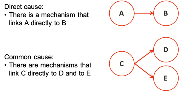
In many cases correlation is related to causal mechanisms (Figure 4):

• There is a mechanism that links one factor to another, so changes in one lead directly to predictable changes in the other. For example, adverse weather conditions that incur clean-up costs might have a direct effect on the time spent on an outdoor activity, so those two sources of unplanned cost are linked.
• A common cause drives two factors, so they are correlated although there is no causal mechanism that links them directly. For example, the costs of two work items might both be driven by the cost of steel or the energy price, although in other respects they might appear to be independent of one another and the commodity prices might not be an explicit part of the deterministic analysis. Another common example arises where uncertainty about the duration of a project drives several overhead costs, and also drives the cost of the project management team.

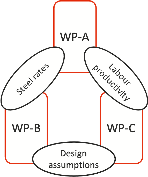
Sometimes the causal links can be complex or messy. For example, the cost of work packages A and B in Figure 5 might be highly dependent on the cost of steel components, A and C might be linked by a common dependence on labour and its productivity, while B and C might both be affected by important design assumptions.

In many cases it is possible to identify the underlying mechanisms that generate correlations. In these circumstances it is better to identify the drivers of correlation (sometimes called ‘risk factors’) and model the mechanisms explicitly than to attempt to estimate correlation coefficients. Rather than using a model that is affected by correlations but makes them hard to see and difficult to represent, this approach makes the factors causing real world correlation the basis of the model, and visible to decision makers, by applying those uncertainties directly to the things they affect.

• The risk factors and the linkages are explicit and easier to explain. This makes it easier to confirm that the models represent what happens in the ‘real world’, and it provides more confidence in the modelling process, particularly for senior managers and people not involved directly in building, testing and validating the models.
• The underlying uncertainty in each risk factor is often easier to estimate and may be linked to a reliable data source. For example, the price of energy may be estimated from market data and trend analysis that is widely available, and then linked to the operating costs of specific business processes through explicit models of energy consumption for the different kinds of equipment they use.

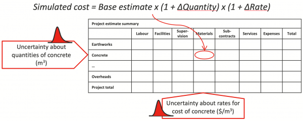
The example of an engineering project in Figure 6 illustrates the approach. Rather than developing uncertainty distributions for each cost type and for many tasks, and then trying to estimate the overlapping influences of uncertainty in labour rates, plant rates, materials costs and so on, it is easier to develop a probability distribution for each of these factors, and then apply them directly to the costs they affect. In a structure like this, the correlations arise naturally when one or more uncertain factors affect several of the costs simultaneously. This is a lot more realistic and easier to explain than modelling the uncertainties in each of the line-item costs individually and then trying to correlate them.

This is easier to understand, easier to build in a model and more realistic than many other approaches to risk modelling for major projects. For further details on this subject, see our resource papers on software project costs here and project budgets here.

Pitfalls in modelling correlation

The existence of correlation does not imply a causal relationship. A causal relationship may be present in some instances, but it cannot be inferred from the existence of correlation. Causal dependency and statistical correlation are therefore distinct types of relationship between two or more entities. Both of them, one of them, or neither might be present.

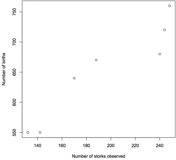
Figure 7 shows a well-known correlation between the number of storks observed in a European town and the number of births. It is not clear that a causal relationship exists, despite the attractiveness of such a notion!

Some modelling approaches are more likely to overlook correlations than others. For example, it is not good practice to use a risk register as the basis of a risk model because many risks are not events but changes from the estimating assumptions that vary continuously across a range and several of them will be driven by the same forces (Figure 6), yet this approach is nevertheless often still seen. There are usually underlying uncertainties affecting a number of the risks in a risk register in a similar way, ensuring the risks are not statistically independent and their effects are correlated, but this is often ignored in models based on risk registers.

Similarly, in relation to modelling based on a list of line-item costs in a budget estimate, there are usually underlying uncertainties that affect several costs in a similar way, such as market conditions, design detail, weather or project duration. Line-by-line modelling of this kind is not recommended.

Selecting realistic correlation coefficients is particularly troublesome when more than one set of correlated uncertainties are interrelated, such as was shown in Figure 5. As well as the difficulty in assessing individual correlation coefficients discussed earlier, the overlapping factors in this example must hold to a precise mathematical relationship because of the cycle from the first to the second to the third and back to the first. In practice, simulation software often overrides any selected correlation coefficients to force them into values that are mathematically consistent with one another. These enforced changes are artificial and have no basis in the analysis. Accepting this fix undermines the integrity of the analysis.

Conclusions and lessons

If the numbers generated by quantitative models are to be used to support important decisions, then they need to be reliable, and executives must have confidence in them. Where the models include uncertainty, the way in which correlation is addressed can have significant effects on model outputs, so real world linkages and correlation between input distributions must be included appropriately. If correlation is ignored, or not treated properly, material errors can be made. If the numbers matter, then they need to be correct.

Using correlation coefficients in models is difficult, unless there is good historical data from which they can be estimated with confidence. Many people find correlation coefficients difficult to understand, they can be very hard to estimate reliably, and they may interact in unexpected ways in models due to the mathematical rules that ensure consistency. Where possible, only use correlation coefficients based on statistical analysis of data; if reliable data does not exist, then use another approach.

Developing bounds on the overall effects of correlation, by running two simulations with and without correlation, provides an initial guide on whether correlation matters. Very often correlation does matter, particularly for decisions that rely on numbers derived from the tails of the output distributions.

Modelling the drivers of correlation explicitly is the easiest and most reliable way of including correlation in quantitative models.

• Models are easier to construct, as the structural relationships are explicit
• This makes the models easier to validate
• The explicit structure and the relationships between important model factors are easier to communicate to others, which increases confidence in the approach and the numbers it generates
• No (or few) correlations must be estimated directly, which avoids the conceptual problems of understanding what correlation means and estimating the values of coefficients; only the distributions of the risk factors need to be estimated, and these are usually more tangible and there is often useful historical information available about them
• The approach works for many kinds of models.

In our work we apply risk factors frequently across a range of models, including:

• Models where the calculations involve primarily multiplication and addition, such as project cost estimates
• Network models, such as those used for project schedules and milestone estimates
• More complex integrated models of project value.

They provide a flexible approach, and they help to avoid most of the difficulties and pitfalls associated with modelling correlation coefficients explicitly.