Extreme project schedule over run
1 Synopsis
There is often a sense that project schedule risk distributions fail to exhibit the long right-hand tails that experience suggests should show up in a realistic assessment of schedule risk. This paper demonstrates quantitatively that unexpected extensions of time might arise not from unforeseen risks or understated risks, nor from a bias towards optimism or over-confidence, but through a systematic interaction between the risks that are taken into account by conventional schedule risk modelling and firefighting behaviour stimulated by schedule slippage.
The mechanism described here shows how growing delays can cascade through a project when:
- Anxiety about poor performance leads to the adoption of inefficient practices, and
- Planning assumptions are undermined as task sequencing and resource timetabling are disrupted.
A simple interaction between straightforward risks affecting a schedule, duration uncertainty, and a degradation of productivity can even generate bimodal distributions of schedule outcomes (Figure 1). Large overruns may arise under modest assumptions about when and by how much productivity will degrade as a schedule comes under pressure. As a project becomes increasingly sensitive to pressure – increasingly fragile – its forecast duration distribution can be changed dramatically.
Figure 1: Effects of increasing fragility
2 Introduction
2.1 Background
Project cost and schedule risk assessment is becoming routine for large projects (Cooper et al, 2014), especially in the engineering and infrastructure sectors. Organisations with good general project planning and management systems that take project risk analysis and modelling seriously might be able to calibrate themselves to the point at which their contingency provisions are realistic and reliable when the characteristics of their projects are reasonably consistent over time.
Where an organisation does not have the corporate memory to enable it to calibrate itself, or where the nature of the projects it implements change, modelling remains a valuable mechanism for exposing risks as well as establishing targets and contingencies.
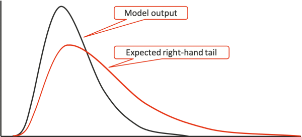
Some concerns about conventional risk modelling remain, even when it is implemented carefully by experienced practitioners. There is often a sense that, while the central region of a modelled cost or schedule distribution, the most likely outcome, appears realistic, the analysis does not give a realistic indication of the potential for an extreme over run (Figure 2). Common sense and experience often suggest that the analysis should show something like the red curve in Figure 2 instead of the black curve.
Figure 2: Understated right-hand tail
2.2 Observed over runs
Most professionals working with major projects for any length of time encounter at least one troubled project that does more than simply edge up to the high end of its forecast duration and cost. If they are not cancelled, these projects might double or triple their budgeted labour hours (Hollmann, 2016, pp61-64). The costs and durations of projects in the mining, petroleum, petrochemical and infrastructure sectors, among others, are strongly linked to the number of labour hours they employ and such a large rise in labour hours will drive an extreme cost or schedule over run.
2.3 Expectations
Attitudes towards extreme over runs are often irrational. Managers generally accept that such things do happen, because they have lived through them, but they always appear to believe there are sound reasons why it will not happen next time.
The only way to make sense of this position is to believe that a forecast distribution of possible outcomes should have a long right-hand tail, as illustrated in Figure 2 - the model output should have included the possibility of a major over run. It is difficult to see how conventional schedule modelling techniques might generate such behaviour though. The fact that it does not arise naturally in quantitative schedule models is sometimes used to suggest that they are flawed or inadequate.
2.4 Reasons for extreme outcomes
In the heat of efforts to limit the damage in a project that is running out of control, there is little appetite for analysing where the problems started. This means that, while there is ample evidence of the effects, there is little objective detail about the causes.
One argument for recurring schedule failures is that the systems and procedures provided to a project team are deficient: in governance, management capability, estimating, planning, procurement, monitoring and control. The common occurrence of projects being initiated with incomplete scope definition, poor quality and patchy estimates or with schedules that bear little resemblance to reality has been documented by researchers (Hollmann, 2016).
Some projects are initiated with plans that can never succeed given the environment in which the team must operate and the resources available to them. It is said by some (Flyvbjerg et al, 2014) that major projects, especially those with a political dimension, are sometimes approved based on cost estimates and duration forecasts that are known to be understated to avoid them being cancelled, so called strategic deception.
Such deficiencies are relatively easy to understand, and well-established professional practices could eliminate the worst of them if those involved admit they exist. There remains a separate challenge, understanding why capable professional organisations find their projects failing, even when their plans have been prepared according to established good practices, have been audited and subjected to critical peer review and risk analysis, and then executed by experienced teams with industry best practice control systems.
2.5 Non-linear system behaviour
A common response to the observation that projects over-run their budgets and schedules is to seek the root causes of the over run. An over run might be blamed on shortcomings in the design, estimating and planning prior to execution, or on events that occurred during execution. All these might have played a role.
Many project professionals have an intuitive understanding that a delay in one area can cascade and disturb work in many parts of a project, but it is difficult to take non-linear effects of this sort into account formally. Acknowledging that it can happen will often be regarded as a sign that the team is not up to the job – after all, their job is to prevent such a loss of control.
The relationship between the durations of individual activities and the overall duration of a project is essentially linear, apart from where activities have multiple predecessors. Even then, if an activity on the critical path extends by a month, we expect the finish of the project to be pushed out a month, one for one. Shortening an activity might not bring the project end date back by the same amount because other activities can then become critical and prevent it, but delays on the critical path will generally flow through day for day. There is a one-to-one linear relationship between slippage in a critical path task and extension of the project finish date.
By itself, the linear relationship between activity durations and project duration cannot generate a long right-hand tail unless there is one uncertain duration that dominates the whole network and is itself heavily skewed or there is one discrete risk that could have little effect or could insert a major delay. In these cases, network modelling might not be as important as examining the dominant activity or the discrete risk. Once there are many uncertain durations of comparable magnitude operating on a complicated network of activities, we see their aggregate behaviour, which will rarely if even exhibit a large amount of skew.
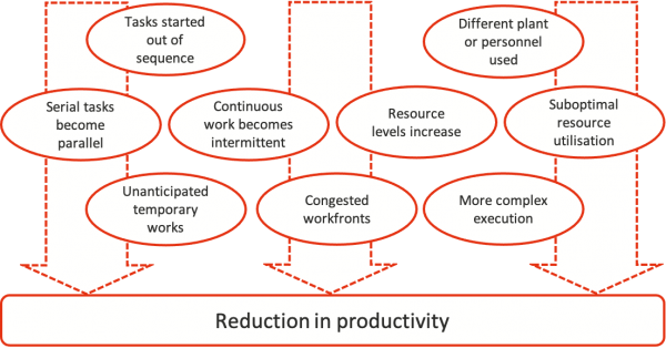
Rather than add to the body of literature that simply catalogues common failings of management and governance, this paper focuses on the point at which most of the problems causing over runs come together, a loss of productivity and consequent increase in labour hours and all that depends on them (Figure 3). This is a simple and familiar non-linear mechanism that affects projects.
Figure 3: Productivity declines - the focus
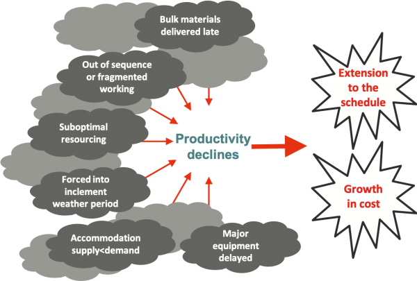
Figure 3 names a few of the factors that can cause a loss of productivity and indicates that many more might be at work. The number of detailed ways productivity can be degraded is limitless. There is no point trying to enumerate and quantify them. A particular project might be delayed by any of them, often more than one. By focusing on productivity itself, it is possible to simplify our understanding of how project schedules blow out.
2.6 Systemic and other factors
As Hollmann (2016) and others have pointed out, the quality of corporate systems, managerial capabilities, leadership and similar matters can be a powerful influence on project success. Where there are sufficient past projects and data to draw on, and they are closely related to projects now being undertaken, relationships between such systemic factors and project outcomes, extracted from historical data, can be used to provide an indication of the contingency requirements of new projects.
Individual project teams are unable to exercise much control over the quality of corporate systems, managerial staff, or leadership. They might draw attention to matters such as decision-making delays, approvals processes that operate on an inflexible timetable, or sluggish in-house procurement and contract management services, but they will not usually be able to change them. All they might do is incorporate allowances for such systemic factors into a project risk model, if internal politics allows them to be open about the issue.
Internal factors such as the availability of requisite skills, plant, materials and access to workfronts might be more within the control of a project. However, factors such as market conditions and interference from existing operations cannot always be overcome. If plans were prepared with a realistic view of the current market for human and other resources and the demands of existing operations, forecasts might take account of these challenges in a realistic way. This is not always the way plans are prepared though.
If asked to describe how such internal and systemic issues will affect a project, attention will usually be drawn to a few isolated areas of the schedule, when in fact the whole schedule is under threat. A focus on isolated impacts cannot explain how delay can grow and spread across an entire project. The next section offers a way to understand this.
3 Firefighting
3.1 Disorderly execution
Project plans are generally based on assumptions of orderly implementation; it is rare for a team to contemplate orderly behaviour being overturned. They think about challenges they face, but they generally assume that they will be able to deal with these challenges in the same orderly fashion they believe will characterise the planned work. This orderly mode of working can break down though.
When a schedule slips and looks set to slip further, pressure to regain control can lead to work being carried out in a different way from what had been planned. As delays begin to mount, it is not uncommon for formal controls to be deliberately relaxed, authority might be delegated closer to the workfront, whether formally or informally, or effectively subverted to enable some progress, any progress, by any means possible. This is a state often referred to as firefighting.
3.2 Responses to disorder
Project plans are optimised to deliver a defined scope as efficiently as possible. Planners arrange to maximise the utilisation of scarce or expensive human resources, specialist facilities and plant.
- If a heavy lift crane is required for two activities, they might be scheduled to follow one another so the same crane can be used for both to avoid unnecessary demobilisation and mobilisation.
- Activities requiring access at heights might be scheduled to follow the completion of steel structures that offer a platform from which electricians, for instance, can operate.
- Construction that will restrict access to an area where major equipment is to be installed might be scheduled after the delivery of the equipment, to avoid having to lift the equipment in with a crane or open a fresh access path where one was not planned.
- A small team of specialist skilled trades people might be scheduled to work over an extended period on several separate areas of a project to avoid a peak in staffing that would put pressure on accommodation and other facilities and to avoid being delayed by lack of scarce skills.
Good planners aim to schedule general works in a sequence that allows each part to be completed as efficiently and realistically as practicable. It follows that, once work slips away from the plan, the project is no longer optimised. The new state will be sub-optimal, and productivity will be lower than had been assumed. Attention will then turn to how the delay can be recovered.
There are many common consequences of schedule slippage and the pressure to recover from it.
- Specialist plant or human resources, perhaps heavy plant or a technical specialist, that were assumed to be available for a particular task are not on hand at the time a delayed task actually starts. In addition to causing straightforward schedule slip, other less efficient ways might be sought to complete the work.
- On a remote site, the availability of accommodation is often carefully matched to the staffing profile of a project, to minimise capital cost. Once work slips, the ability to increase the number of personnel to recover progress can be severely limited. Overflow staff might need to be housed some way from the site and bussed in each day, often losing 20-25% of the working day in unplanned travel.
- A well-integrated crew, working systematically from one area to the next before the pattern of work was disturbed, may have moved on to another project to which they made a prior commitment. A newly formed replacement team who are not familiar with the project will have to be brought up to speed, and they are likely to operate less efficiently than the original crew.
- If a construction activity were to rely on access being provided by earlier works that have now been delayed, such as structural steel providing access to elevated sections of a plant or demolishing a building blocking the shortest way into the site, temporary works might be undertaken to enable the activity to proceed, erecting scaffolding or building a temporary road to enter the site from a different direction. These temporary works will not only incur their own delay and cost but might make it more difficult to complete the task for which they are needed than had been assumed in the original plan. They will often interfere with other activities in the same area, slowing them down as well.
- When IT code or approved system engineering designs that had been assumed would be available on a specified date are delayed, software projects might build temporary code and develop interim designs to allow other tasks to start, just to make some progress, knowing that interfaces or even system architectural features might have to be reworked later, taking additional time.
- Tasks that were to be carried out in series are run in parallel or at least overlap to some extent, possibly giving rise to access limitations and congestion on construction sites that reduce productivity or resulting in redesign and rework as the strict logical dependence of design decisions is not respected.
- Work that was to be carried out by one integrated team as a single unified activity is carried out in disjointed smaller tasks separated in time. This might entail multiple rounds of mobilisation and demobilisation where only one had been expected. It might also lead to an inefficient mix of personnel being set to work because a small team cannot be optimised to provide the required mix of skills and capabilities as easily as a larger one. At the conclusion of the work, there might be unplanned rework required to integrate the separate parts.
The overall path towards lower productivity is outlined in Figure 4.
Figure 4: Responses to schedule slippage
These are just a small number of the expedient measures that might be triggered as a schedule slips. Their common characteristic is that the efficiency or productivity of the work will fall as the original optimised plan is supplanted by alternatives driven by a need to make, and be seen to be making, progress. An appearance of intense activity and people working long hours at least shows they are trying hard.
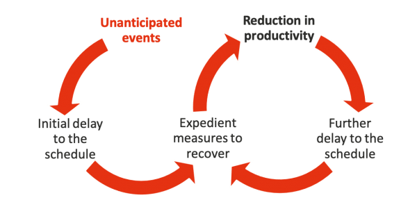
A high-level view of the cycle by which delay, and a loss of productivity can ratchet up is illustrated in Figure 5. Starting with unanticipated events affecting progress on the left, the feedback loop on the right perpetuates and amplifies the impact on a project.
Figure 5: Cycle of escalating delay and declining productivity
Unless there is a deliberate effort to stand back and replan the job as carefully as it was planned at the outset, as soon as plans for a significant part of the work are disrupted, it is unlikely ever to be as efficient as originally envisaged. Replanning usually involves setting revised targets and might require deliberate and explicit trade-offs between cost and schedule.
Such root and branch re-evaluation is rare. Major projects have a momentum of their own and there are barriers to acknowledging they have run into difficulties, not least personal and political embarrassment.
To explore how a loss of productivity could propagate through a project, we conducted an experiment using a Monte Carlo simulation of several model project networks derived from real projects. This is described in the following sections.
4 Modelling productivity loss
4.1 Initial concepts and definitions
To explore how the mechanism illustrated in Figure 5 could affect the schedule of a project, we constructed models of real project networks in Excel with the @RISK add-in. The models were based on information extracted from schedule risk models built originally in Primavera Risk Analysis (PRA).
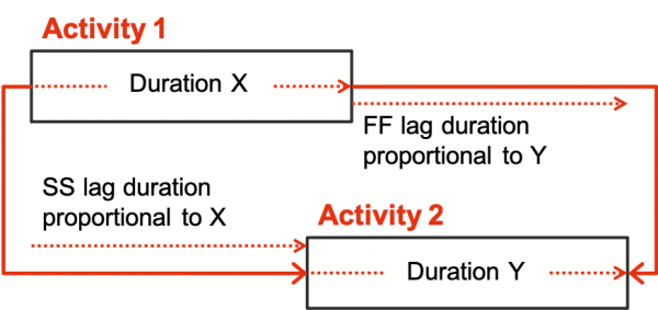
Activities were linked as they were in the original network by Finish-Start (FS), Start-Start (SS) and Finish-Finish (FF) logic. @RISK distributions were applied to the task durations to represent their possible variation. Variations in the durations of lags on SS and FF links were made to vary in proportion to the variations in the duration of each lag’s predecessor for SS links and successor for FF links, illustrated in Figure 6. This logic replicated the working of a conventional PRA project schedule risk model.
Figure 6: Uncertainty in lag durations
Next, each activity’s duration was adjusted according to how late it started compared to when it was initially planned to start, to represent the effects of the factors discussed in Section 3.2. In practice this relationship will be complicated and different for different parts of a project; this model is not intended to be used for prediction but simply to explore the mechanism.
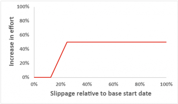
The effect of disruption arising from schedule slippage in each individual activity was modelled with the simple relationship shown in Figure 7. Slippage, the horizontal axis, is defined in Figure 8.
Figure 7: Effect of slippage on effort
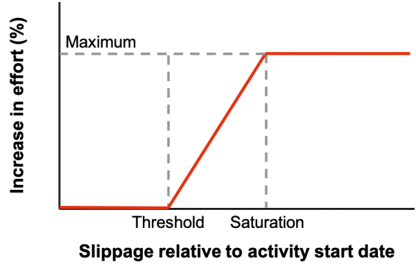
Figure 8: Definition of slippage

In the models, activities were subject to simple duration uncertainty used in common schedule risk models. In addition, their durations were extended according to how late they started relative to the date on which they were planned to start.
The horizontal axis in Figure 7 represents the slippage ratio shown in Figure 8. The vertical axis shows the extra effort required to complete the task as a percentage of the effort if the activity started when planned. Unless a project has scope to put on additional people, plant, accommodation and other facilities, a loss of productivity will translate into an extension of time.
The form of the relationship in Figure 7 is based on the premise that:
- Below a certain threshold, slippage will be managed within the original plans and work practices, so there might be delays but no major change in the way work is carried out, which is the usual premise of risk modelling
- As the slip grows beyond that threshold, extra time is required as productivity declines
- There comes a point at which the project has settled into a new mode of operation, a less ordered state than was intended, neither getting worse nor returning to the well-ordered optimised state assumed in the original plan, the saturation point.
This definition of slippage in Figure 8 takes into account the effect of delays arising at different stages in a project. A two week slip after a month of execution, when Slippage = 50%, is likely to be more disruptive than a two week slip after a year, when Slippage = 2%. The impact of the level of slippage is determined by the Threshold, Saturation and Maximum parameters in Figure 7.
Productivity uncertainty is often a key source of risk in major projects. That is a separate matter from the mechanism being described here. The mechanism examined here concerns how the productivity that would otherwise be expected, subject to any inherent uncertainty about its level, can be degraded simply because work slips from the planned schedule and the consequential effects of firefighting outlined in Section 3.
In the models, an activity’s duration was calculated as shown in Figure 9, where the base duration is that in the initial plan, the duration distribution represents the relative effect of risks and risk factors on the duration, as in a conventional risk model, and the increase in effort is the effect illustrated in Figure 7.
Figure 9: Activity duration formula

4.2 A simple illustrative example
To see how this effect can build up in a project, consider the simple sequence of activities in Figure 10, where durations are displayed in weeks. (This is only to illustrate the mechanism by which delay can not only pass on to later activities but become increasingly severe if it triggers a loss of productivity by delaying later tasks. Examples based on actual project schedules are discussed later.)
Figure 10: Simple example
The profile shown in Figure 11 has a threshold of 12.5%, a saturation point of 25% and a maximum impact of 50%. These parameters could represent a project where:
- Slippage of up to six weeks in a year will be handled without changing the fundamental operation of the project or losing productivity, affected only by the usual risk model uncertainties
- Slippage above six weeks in a year will have an increasingly disruptive effect on each activity’s duration the worse it gets, until it reaches 25% of the time between the start of the project and the activity’s planned start date
- Once slippage reaches 25% of that period between the project start and the planned start of the activity, the impact on productivity will become no worse because the project will settle into a new tempo of operation, but activities started after that point will take 50% longer than originally planned.
Figure 11: Productivity loss profile
If each activity is affected by an equal level of risk and all durations are extended by 13% over their base levels, leaving aside the productivity effect, the activities are all extended by 13%, shown by the yellow bars in Figure 12. However, when this extension is combined with the sensitivity in Figure 11, noting that 13% risk impact is only just above the 12.5% threshold point, their durations extend far more, shown by the red bars in Figure 12.
Figure 12: Example - Risk and productivity impacts
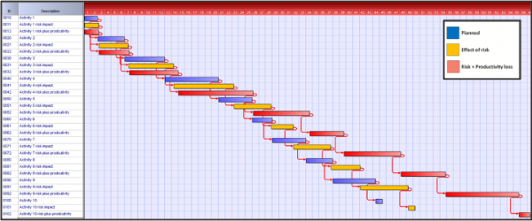
A project with a general schedule risk level sufficient to extend durations by 13%, requiring a 13% contingency, blows out to an overall duration 50% longer than its base level, a 50% contingency. If that were to be assessed as a contingency, it would be nearly four times larger than initially thought, 50% compared to 13%. No additional uncertainty has been introduced, just a mechanism by which slippage causes productivity to decline.
This is not an attempt to model the behaviour of a real project. All the human and information systems that affect real projects would be impossible to represent and the effort is unlikely to yield useful information for a specific project. However, it demonstrates that a simple and plausible mechanism could make a project schedule slip far more than an initial examination of risks would suggest.
An experiment with this mechanism using real project networks is described in the next section.
5 Testing real schedules
5.1 Approach
The simple example in the previous section illustrated the mechanism by which productivities might reduce and schedules extend. To examine the effects on real projects, we extracted several high-level project networks from prior schedule analyses into Excel, recreating the logical structure of each network. The focus of this investigation was the effect on the schedule of a loss of productivity interacting with the probabilistic effect of risks, as described above.
We developed three versions of each network model:
- A deterministic calculation, the duration that a conventional planning tool would yield
- A probabilistic calculation in which duration distributions were applied to the activity durations, which mirrors normal Monte Carlo simulation schedule modelling
- A probabilistic calculation in which duration distributions were applied to the activity durations, as in the previous case, and then each activity’s duration was also made to depend on how late it started compared to when it was initially planned to start, to represent the effects of the mechanism in Figure 7.
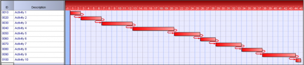
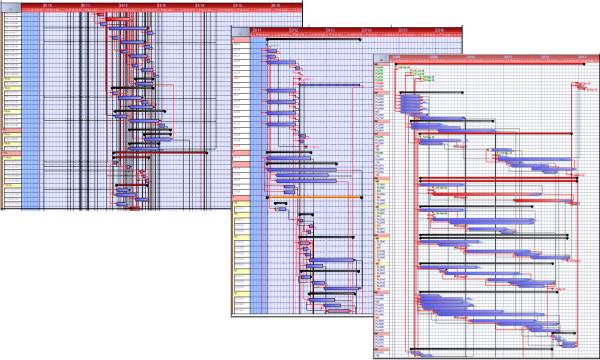
To illustrate the nature of the networks examined, a single page from the Gantt chart of each of three of the models is shown in Figure 13. They vary in their overall scale and the density of links between activities. The networks are all based on real projects; we have stripped identifying information and changed the activity coding to avoid disclosing their sources. The details do not matter; these are real network structures with no extraordinary characteristics.
Figure 13: Model Gantt chart sections
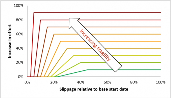
A range of productivity loss profiles was used, ranging from perfectly robust to extremely fragile, illustrated in Figure 14. Each step from the lowest (green) to the highest (red) profile can be thought of as an increase in the project management system’s fragility, in the sense that it starts to degrade at a lower slippage threshold, the maximum degradation increases and the maximum is reached more quickly from one profile to the next.
Figure 14: Intermediate profiles
The schedule models were simulated with one hundred profiles. For each profile, the model was evaluated through one thousand iterations.
5.2 Results
General results
When the productivity effect was cancelled out, the models generated overall duration distributions consistent with those produced by a conventional schedule modelling tool, demonstrating that the networks were transferred successfully into Excel. The examples in this section are from one of the model networks illustrated in Figure 13.
The model’s probabilistic output, with no productivity loss, just the effect of risk, is shown in Figure 15 as a histogram of results expressed relative to the deterministic duration of the project, which is represented by the 100% point on the horizontal axis.
Figure 15: Probabilistic results – effect of risk alone
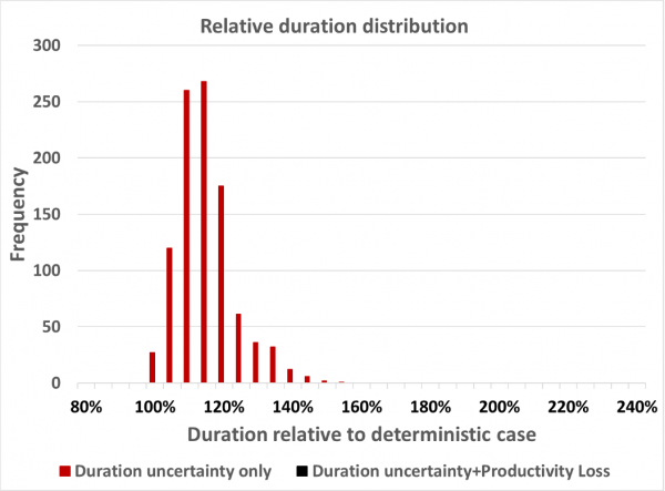
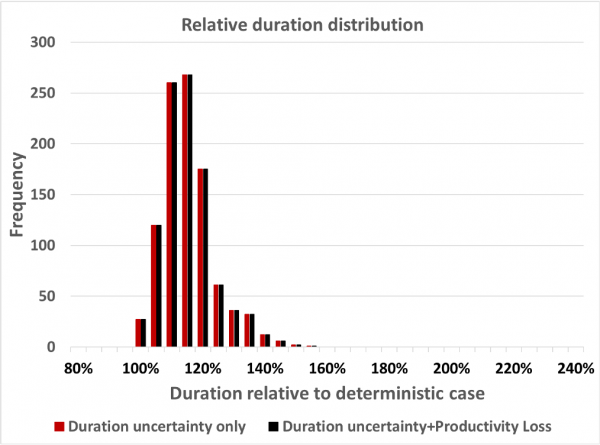
For an extremely robust case, as expected, the productivity loss models give the same results as the deterministic model, illustrated in Figure 16.
Figure 16: Productivity loss model – robust case
As an example of a very fragile case, we examined a profile with Threshold = 0%, Saturation = 5% and Maximum = 80%. Figure 17 shows that the productivity loss model diverges markedly from the probabilistic model.
Figure 17: Productivity loss model – fragile case
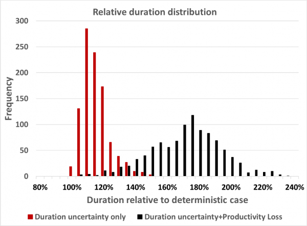
There is still a small chance that the project will remain under control, but the vast majority of the simulations generated a large overall schedule extension. Once the delays start to set in, the effect cascades through the network and causes extensions of time over and above anything caused by risk. It shifts the entire distribution to the right.
This is a phenomenon that is observed in practice, sometimes referred to as a blowout (Hollmann, 2016, pp61-64 and 279-290). Some projects cascade into greater and greater delays as soon as they start to slip. They are very fragile.
The first activity to run late might disturb subsequent work a little. That small disturbance is amplified by the effect illustrated in Figure 7, so later activities are disturbed by a relatively larger amount. This is then amplified by the greater loss of productivity in subsequent activities and so on through the course of the work. Work slips from the baseline by a larger percentage at each stage, not just the same proportion as earlier slippage.
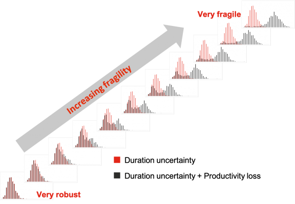
The progression from robust to fragile can be seen in Figure 18.
Figure 18: Effects of increasing fragility
While a realistic quantitative analysis of the behaviour being considered is not a practical proposition for routine project management, the qualitative nature of these results is instructive. It shows that if productivity degrades as a project’s schedule slips, the project’s duration distribution may be quite different from what a standard analysis would suggest.
Some features of the distributions in Figure 18 stand out. As a project becomes more fragile, less able to resist the firefighting that reduces productivity, its outcome distribution changes shape. A small amount of sensitivity causes a long right-hand tail to develop.
The potential to generate a long right-hand tail offers one explanation for the feeling among some project professionals that conventional risk models fail to capture the potential for projects to experience extreme over runs. A loss of productivity due to firefighting triggered by progressive slippage will produce such behaviour.
Other explanations offered for risk models failing to exhibit long tails or blow outs include:
- That the estimates of possible variation, the source of the risk model inputs, fails to capture extreme skew due to unwarranted optimism or because participants are reluctant to accept the possibility of very poor outcomes due to pride or fear of speaking out
- Omission of the influence of systemic risk factors such as poor management capability, inadequate scope definition, flawed estimating and planning practices or optimism about novel technology (Hollmann, 2016), the absence of features that could prevent the initial harm to the schedule or restrain the descent into firefighting once a schedule starts to slip
- The effect of so-called unknown unknowns.
The mechanism described here will be stimulated by anything that causes a schedule delay. A link between productivity and schedule slippage amplifies anything delaying the schedule and explains nonlinear behaviour in a straightforward manner, without postulating anything more than the straightforward mechanism outlined in Section 4.
Moderate fragility
Severe stress can be envisaged even with a modest sensitivity to slippage. The mid-point in the profiles evaluated here is illustrated in Figure 11, the red line. It has a threshold of 12.5%, saturation of 25% and maximum additional effort or duration extension of 50%, the vertical axis.
This profile causes the overall project duration for one of the networks to have the extended right-hand tail shown in black in Figure 19. The left-hand peak of the black histogram represents a good outcome where work does not slip enough to trigger a runaway productivity loss. The right-hand tail represents a poor outcome where, once slip began to appear, the project does run away and the delay is not recovered.
Figure 19: Effect of moderate sensitivity to slippage
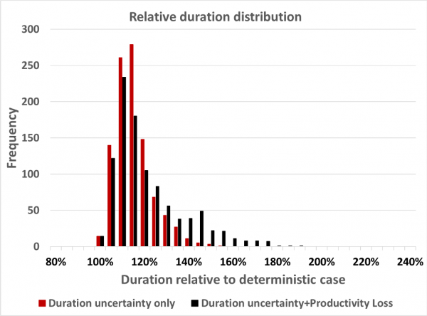
It is worth noting that, even though the peak of the red histogram represents a project maintaining control and avoiding firefighting, it could entail a schedule slip of more than twice the amount commonly allocated as a contingency, the value near the peak of the red histogram. The impact of uncertainty, in ‘standard’ risk management, remains a real concern whether there is a loss of control or not.
The same fragility parameters, applied in one of the other networks, generate distinctly bimodal behaviour (Figure 20).
Figure 20: Bimodal duration distribution (second network)
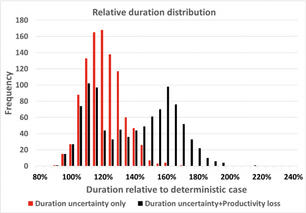
The distribution does not just stretch out uniformly, it becomes bimodal. This behaviour is discussed by Hollmann (2016 Fig 4.7). If things start to go wrong, they go badly wrong. There are no half measures. Work either proceeds roughly as expected, subject to the identified risks, or it flips into a different mode with a marked overall delay.
There is always a chance that a project will remain under control despite being susceptible to a loss of productivity, the left-hand section of the black histogram. This will happen if the impacts of the uncertainties affecting the project are not large enough to trigger the slide towards chaos. If those impacts are large, it will slip into a different mode, the right-hand section.
This is not due to anything that would normally be included as a risk in a conventional analysis or any exotic distributions being used for the durations of individual activities. It is just the systematic effect of the pressure arising from schedule slippage causing a change in plans and behaviour that leads to reduced productivity further downstream. It is not a probabilistic effect but an interaction between probabilistic variations and management action, or inaction, when the schedule slips, a descent into chaos.
6 Related matters
6.1 Project cost
There will usually be a trade-off between cost increase and schedule extension in a project. Money can often be used to recover or prevent slippage and schedule performance can sometimes be sacrificed to save money. That has not been addressed here.
Common sense suggests that if a major project’s schedule is slipping into the right-hand region of the black histogram in Figure 19, additional costs will be incurred simply due to the schedule extension – extending the schedule will drive increases in overheads and other time-dependent costs. In addition, efforts to recover the slippage, or at least prevent it from getting worse, are likely to incur further unplanned costs.
The pronounced slippage and bimodal behaviour seen here would almost certainly be reflected in the cost outcome of a project as well as its schedule. If the mechanisms described here can affect a project, they will give rise to the potential for an unexpected cost overrun as well as an unexpected schedule extension.
6.2 Management responses
This experiment does not purport to represent a project in detail. Nevertheless, the concept of a cascading loss of productivity can be contemplated by any project and some common-sense responses are clear.
The emotional barrier to accepting that a plan has been overtaken by events and has the potential to run out of control is usually quite high. No one, from the work area supervisors through to the project management team, their managers and the project’s owners, wants to admit that control might be slipping. There is often a preference to wait and see if the slip can be recovered.
However, in the absence of a way to eliminate the risks that trigger the process (Figure 5) entirely, the only way to avoid the danger is to:
- Recognise that it can happen
- Be alert for early signs of slippage and firefighting creeping into the project
- Be prepared to deliberately reset a project, or part of a project, rather than have it happen by default, to restore order and prevent the development of chaos.
7 Conclusions
The purpose of this exercise was to gain a qualitative understanding of whether the stress caused by delay, cascading through a project as reduced efficiency, could interact with straightforward schedule logic and duration uncertainty to amplify the delay.
The modelling described here demonstrates that large extensions of time might be explained without invoking unforeseen risks, optimistic estimating or wilful deception. It can be explained by a systematic interaction (Figure 5) between:
- The impact of recognised risks that are usually addressed by a conventional risk analysis
- Firefighting behaviour, causing a loss of productivity, stimulated by concern about delay.
There might be other factors at work as well, but it is not necessary to assume that major risks have been overlooked to believe that a project can slide into a major overrun. The slide can take on a life of its own during project execution. Whether that will be felt as an extension of time or additional costs is a separate matter.
The mechanism described here shows how growing delays can cascade through a project as each activity is placed under increasing pressure by delays in the activities that came before it. The pressure will lead to:
- Anxiety about poor performance, resulting in the adoption of inefficient practices, and
- Planning assumptions being undermined when task sequencing and resource timetabling are disrupted, so that revised plans are less efficient than the original.
The fact that projects suffer when their schedules slip, so that plans have to be changed, is not a fresh insight in itself. The concept that the effect can build up and propagate systematically through a project via a quantitative mechanism offers a useful new mental model for thinking about control during project execution. It points to the need to be alert for changes in management behaviour that might indicate the start of a slide into firefighting behaviour and to be prepared with actions that will re-establish order and control.
8 References
Cooper, DF, PM Bosnich, SJ Grey, G Purdy, GA Raymond, PR Walker and MJ Wood (2014) Project Risk Management Guidelines: Managing Risk with ISO 31000 and IEC 62198. John Wiley and Sons, Chichester. ISBN 978 1 118 82031 5.
Hollmann, JK (2016) Project Risk Quantification: A Practitioner’s Guide to Realistic Cost and Schedule Risk Management. Probabilistic Publishing, Gainesville FL, ISBN 978 1 941075 02.
Flyvbjerg, B, M Garbuio, and D Lovallo (2014) Better forecasting for large capital projects. McKinsey & Company Strategy & Corporate Finance, 1 December, last accessed from here.