Beta PERT origins
Background
The Program Evaluation and Review Technique (PERT) (Malcolm et al, 1959) was initially known as the Program Evaluation and Review Task. The task to which this refers was assessing the uncertainty in the plans for the development schedule and cost for the Polaris weapon system. The word ‘task’ was later replaced by ‘technique’ when the method began being used on other projects but the initials remained PERT.
The team who developed the method wanted to know the mean and variance of the duration of the activities making up the Polaris program. They wished to use these to calculate the mean and variance of the critical path duration of the entire program.
It was not reasonable to expect the program engineers to assess the variance of their duration forecasts. Humans have no intuitive sense of the variance of an uncertain quantity and even assessing the mean is a challenge.
They decided that they could ask engineers to estimate optimistic, most likely and pessimistic durations, a three point estimate, and seek to derive the mean and variance from these values. They required a mechanism to convert a three point estimate into an equivalent mean and variance and settled on using a modified Beta distribution that would have the same minimum, mode or most likely and maximum values as the forecast and from which the mean and variance could be derived.
Beta PERT
In the decades since PERT was first developed, the Beta PERT distribution to which it gave rise has come to have a special place in risk modelling. Many people assume that it must represent a fundamental characteristic of uncertainty in durations and other features of projects. In fact, the rationale for using a Beta distribution is anything but fundamental.
The team were not concerned with the mathematical form of the distribution so much as finding a way to assess the mean and variance of the individual activity’s distributions. From these they calculated the mean and variance of the critical path as the sum of the means and variances of the activities on the critical path. The overall mean and variance were used to approximate the distribution of the program’s duration.
As an aside, there are several problems with this approach to assessing the overall program duration. The main one is that it concentrates on a single path through the network and takes no account of the possibility that parallel paths could become critical. It also ignores correlations between activities. These are serious issues for modelling but do not affect the way the Beta PERT distribution was used to convert three point estimates into a mean and variance.
Choice of Beta
The choice of the Beta distribution is explained by the mathematician on the original PERT team (Clark, 1962) in the following way.
The author has no information concerning distributions of activity times, in particular, it is not suggested that the beta or any other distribution is appropriate. But the analysis requires some model for the distribution of activity times, the parameters of the distribution being the mode and the extremes. The distribution that first comes to the author’s mind is the beta distribution.
He goes on to explain that one of the features of the Beta distribution that makes it an attractive choice is that the mathematical manipulation of the distribution is manageable.
Derivation of mean and variance
The team knew that, to help the engineers assess the uncertainty in their activity’s durations, they were starting with a three point estimate. They needed to convert those three points into a mean and variance and, for convenience, Clark selected a Beta distribution to do this.
Clark further explains that three values, minimum, mode and maximum, is not enough to completely define a Beta distribution and a further assumption is required to permit the three point estimate to be converted to a mean and variance. By analogy with a Normal distribution, in which almost all outcomes (99.73%) fall within plus or minus three standard deviations of the mean or a range of six standard deviations (six sigma), he assumed that the range between the minimum and the maximum values of a forecast represents six standard deviations of the duration’s distribution. This defined the variance, the square of the standard deviation, and fixed the Beta distribution’s shape parameters.
Even once the Beta distribution was defined by the three point estimate and the six sigma assumption it was still a challenge to derive the mean analytically as it required the solution of a cubic equation, but a simple approximation was found to be a good fit to the exact solution. Using this approximation and the six sigma assumption, what we know as the Beta PERT distribution was defined. It is specified by three values, the minimum A, the mode or most likely value M and maximum B and has a mean and variance calculated as follows.
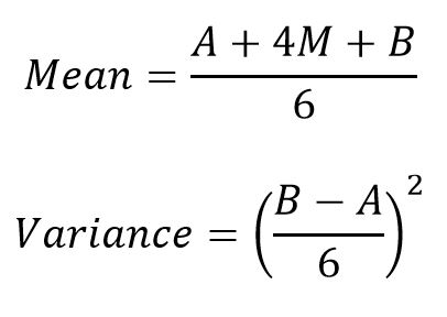
The equation for the mean is an approximation to an exact solution and the equation for the variance is based on an approximate analogy with the Normal distribution.
Current implementations
The mathematical challenges that drove these decisions over fifty years ago are no longer relevant given the computing power we now have at our disposal. Despite this, the Beta PERT has been used to build project risk models for so long that it has become part of the furniture, leading many to believe that it is in some way the natural or correct distribution for this type of work. In fact, its use for project modelling has no fundamental mathematical, statistical or empirical justification. It was a sound pragmatic solution to a computational requirement in the days before computers were as powerful and widely available as they are now, not a statement of the true form of project activity duration uncertainty.
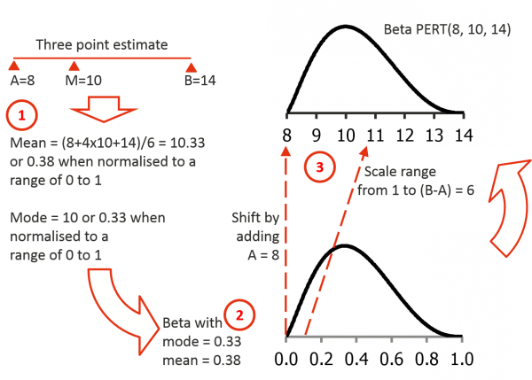
Modern modelling tools implement the Beta PERT in a way that mimics the characteristics used in the original PERT analysis using a standard Beta distribution as a base, as shown in Figure 1. The two parameters required to define an underlying Beta distribution are chosen to place its mode and mean at the same relative positions between zero and one as M and the mean, calculated using the formula above, are between A and B (step 1). The underlying Beta distribution on which the Beta PERT is founded runs from zero to one (step 2). This is shifted by adding to it the minimum value A; it is also scaled to span the range A to B (step 3).
Figure 1: Generating Beta PERT from Beta
Conclusion
The modern Beta PERT is a reverse engineered replica of the distribution chosen for convenience in the 1950s to convert three point estimates into a mean and variance.
It might be argued that the Beta PERT would not have stood the test of time if it did not offer something useful. For the purposes of project cost and schedule modelling, it has a satisfying smooth shape, as opposed to the unnatural angular shape of the triangular distribution, and it can represent skew. That is all.
References
Clark, CE.,(1962), “The PERT model for the distribution of an activity time”, Operations Research, 10, 405-406.
Malcolm D.G., Roseboom J.H., Clark C.E., and Fazar, W., (1959), “Application of a technique of research and development program evaluation”, Operations Research, 7, 646-669.