Introduction

This tutorial is drawn from Broadleaf’s long experience with project range analysis, also referred to as quantitative risk analysis or probabilistic risk analysis. It describes some key lessons about project range analysis, and what constitutes good practice. The material covers the analysis of both costs and schedules; the same principles apply to both.

Range analysis

Overview

The range analysis process has six steps, each of which is discussed briefly in the following sections:

1. Understand the risks
2. Construct a quantitative model and identify the inputs it requires
3. Gather inputs and run the model
4. Check and validate the model
5. Reconcile the outcomes with reality
6. Revise the model and its parameters as necessary

The steps for cost and schedule range analysis are similar. Where there are important differences, they are noted in the discussion.

Step 1: Understand the risks

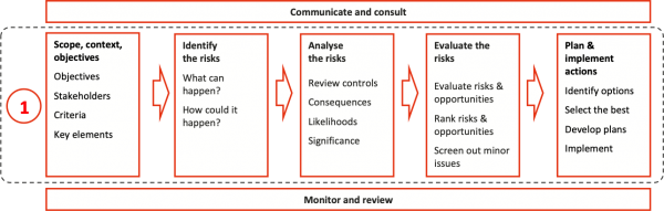
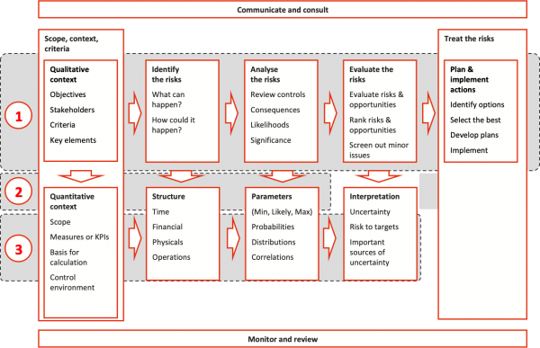
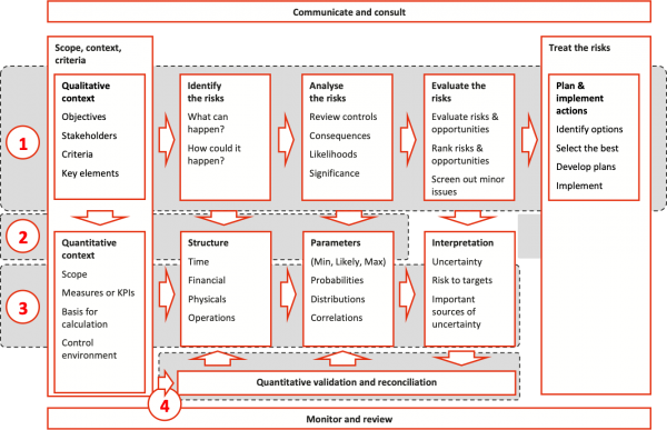
The purpose of this step is to gain a broad recognition of the uncertainties we need to take into account. The approach usually follows standard company practices, using workshops and generating risk registers. In our work, it is usually aligned with ISO 31000 (Figure 1).

There are several potential pitfalls of which you should be aware, so you can avoid them as far as possible:

• Complacency: even if the project seems to be ‘routine’, it is important to take it seriously and to assess all the relevant risks
• Group think: use a diverse group of people in workshops, with different backgrounds, so that all the main assumptions are questioned and tested
• Confusion between project and business responsibility: all sources of uncertainty should be identified, so relevant ones can be included in the quantitative analysis that follows.

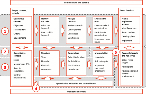
Step 2: Construct a quantitative model

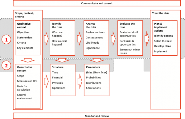
The purpose of this step is to build a quantitative model that is appropriate for the analysis and to identify the information that will be needed for it (Figure 2).

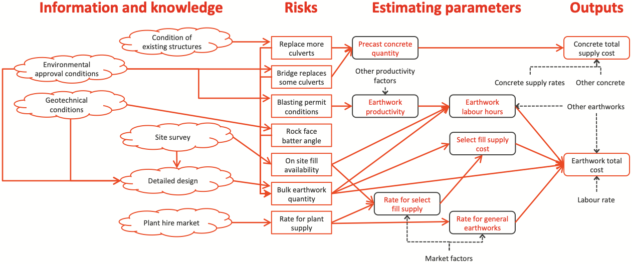
Building useful and valid models is not easy. It requires a sound understanding of the main risks, the centre column in Figure 3, and the underlying sources of uncertainty and their relationships, on the left. This understanding leads to a set of estimating parameters, on the right, that combine to represent the combined effects of the uncertainties, on the cost in this case.

The example in Figure 3 illustrates concrete and earthworks costs. The same principles apply for all cost and schedule models: understand the main sources of uncertainty and what influences them, and then identify appropriate parameters that allow the desired outputs to be calculated. The sources of uncertainty, the left hand side, are often complicated and interact with one another. Distilling them into factors that can be used for calculations involves judicious approximations, a focus on the dominant factors and rigorous attention to the structure of the calculation, the model, to ensure that it is realistic.

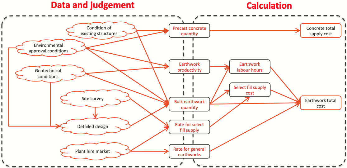
The risk structure in Figure 3 can be simplified to illustrate the development of a workshop and model structure like Figure 4. The main items to be estimated are in the centre column of Figure 4; they are estimated using specialist judgement, supported by data where it is available, about the influencing factors on the left; model calculations are on the right hand side. The selection of the risk factors must ensure that it will be possible to make realistic calculations, separating distinct sources of uncertainty and generally reflecting the structure of calculations made in the preparation of an estimate or schedule.

No model will be absolutely comprehensive and precise. Judgement is required to determine which aspects of the uncertainty in a project should be incorporated in a model and how this should be done.

For a cost range analysis:

• Develop the model framework in a spreadsheet, possibly building on past models
• Separate independent sources of uncertainty (quantities, rates, productivities, areas of work with different characteristics)
• Summarise the costs to allow uncertainty factors to be applied cleanly across the model, perhaps as shown in Figure 5
• The information required will include ranges for the most important quantity, rate and productivity drivers.

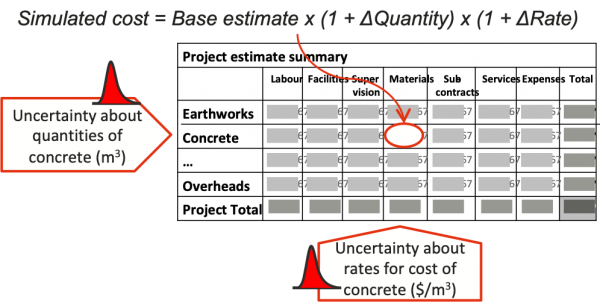
This general form has proved to be an effective basis for cost modelling in many sectors. The rows are generally associated with uncertainty in the quantity of work in each major part of the project. In mining and engineering this will often be along the lines shown in Figure 5. In a design task or software development it might be the major components of the project. The columns are generally associated with different categories of costs – such as labour, materials, equipment, contractors’ fees and freight – where the unit costs in one category are subject to uncertainty that is different from that affecting the other categories.

For a schedule range analysis:

• Develop the model framework in a scheduling tool like Primavera Risk Analysis (PRA) or Safran Risk
• Separate independent sources of uncertainty (blocks of closely related work, quantities, productivities, rates, areas with different characteristics)
• Aim for a high level but logically linked network, at a level of detail that might be appropriate for a Board presentation
• The information required will include the schedule network logic, durations and ranges for activities or for factors affecting durations such as productivity and quantity uncertainty.

For an integrated cost and schedule range analysis, time-variable costs and the way schedule variation will affect them must be identified too. Cost and schedule integration can be as simple as implementing in a cost model the schedule distribution generated by a schedule model. It can be addressed in more detail up to the level of time dependent and time independent costs in individual activities. Judgement is required to determine the most appropriate level of detail, the level at which the model provides useful insight without absorbing an undue amount of effort in development, running the model and interpreting the results.

Pitfalls for cost range analysis include:

• Too much granularity, leading to several independent elements of the model embodying the one source of uncertainty, is inefficient as it results in multiple assessments being made of essentially the same thing, and the separate factors generally have to be correlated in the model if they are to be realistic, which can be difficult
• Too little granularity, when one factor wraps up several different sources of uncertainty so one factor represents a complicated mix of risks, making it difficult to assess and requiring complicated correlations to be used in the model
• Confusion about what project-level contingency has to cover and what is a business-level matter, such as regulatory changes.

For schedule range analysis, pitfalls include:

• Gaps in network logic, such as activities with no predecessor or no successor, dates that are fixed rather than being dependent on the durations of activities in the plan, or scheduling activities to fall as-late-as-possible, so they float and have no effect on the modelled duration
• Confusion about responsibilities for important dependencies, such as approvals to proceed, close downs, tie ins, cut-overs, and so on.

A pitfall common to all forms of range analysis is to use too many factors and ranges. A balance must be struck between the level of detail (the number of factors) and the effort required to generate useful estimates in Step 3. While it may seem counter-intuitive, additional levels of detail do not always lead to more accurate or useful outcomes. If there is too much detail, model structures become complex, identifying and managing correlation becomes difficult, and the outcomes become much harder to analyse and interpret.

For a schedule model, 30-100 activities works well if you construct a model network and align it with the main schedule.

• Release all constraints apart from approval to proceed or equivalent, except where key dependencies have no predecessor, such as a major external dependency like being granted access to a site, by an independent party, to begin work
• Logically link as-late-as-possible activities, and identify what will really trigger their start
• Build uncertainty into remaining dependencies that the project has to accept, representing the uncertainty in external events on which you depend; Figure 6 shows an example of how this might be done in PRA.

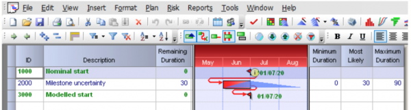
In the example, the range of dates at which the milestone is expected to fall is from 30 days earlier to 60 days later than the nominal date. Uncertainty of this sort can be modelled as follows:

• Create a milestone uncertainty activity (#2000) with a base duration of 30d and a 7 day calendar
• Link the milestone uncertainty activity Finish to Start from the nominal start (#1000) with a negative 30d lag so its completion falls on the same date as the nominal start
• Apply a distribution with parameters (0d, 30d, 90d) to the milestone uncertainty activity
• The base duration cancels out the negative lag in a static view, so the dates of successors are preserved for easy reference
• Variation in the milestone uncertainty activity causes the modelled start (#3000) to move between 30 days early to 60 days late while being most likely to fall on the nominal start date.

When combining activities in a schedule model, there are several ways in which to handle groups of tasks with related uncertainties;

• Assess each group as a whole, allocate uncertainty pro rata to individual activities, and then correlate their distributions
• Use a single risk factor, a stand-alone distribution typically expressed as a percentage variation, to represent the relative aggregate variation and apply it to all activities in the block, which has the same effect but is usually faster and leaves less scope for transcription errors
• Use risk factors to represent uncertainties in inputs to durations (such as quantities, productivities, linear rates of advance) and apply the required combination of factors to each activity.

Step 3: Gather inputs and run the model

The purpose of this step is to gather data to populate the model and produce initial outputs (Figure 7).

Inputs are commonly generated in a range analysis workshop, covering the structure established in Step 2. We usually use a template like Figure 8, which is structured to avoid systematic bias as far as possible.

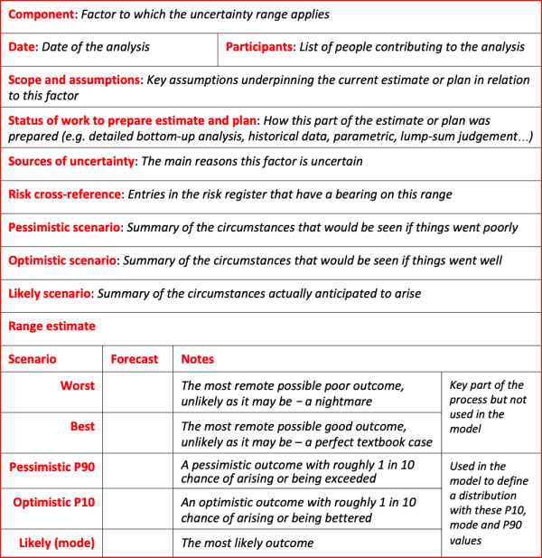
A common pitfall is to attempt to quantify too many factors in the time available for a workshop. We use a rule of thumb of 15-20 minutes for discussion and analysis of each factor.

Step 4: Check and validate the model

The purpose of validation is to pick up errors in the model, unrealistic input ranges or unrealistic prior expectations that the model will challenge, and so build confidence that the model is realistic (Figure 9).

Several approaches may be used, often in combination:

• Compare outcome with expectations, benchmarks and experience, and investigate if the outcomes ‘don’t smell right’
• Discuss and diagnose apparent anomalies with estimators, planners, managers and specialists
• Conduct sensitivity analyses
• Undertake detailed model audits if anomalous outcomes persist.

Robust model validation should always be undertaken, to help avoid common pitfalls, which include:

• Adopting an uncritical approach to models, amounting to blind faith in their veracity and the outcomes they generate
• Having unrealistic expectations of what a model can do and the accuracy of its outcomes
• Misunderstanding the effects of nodal bias in schedule networks, and the associated non-linear effects on overall durations.

Step 5: Reconcile the model outcomes with reality

The purpose of this step is to gain acceptance for unexpected or unwelcome findings, by demonstrating why the outcomes align with reality and are logical consequences of the model (Figure 10).

Discussion and diagnosis of anomalies and examination of sensitivity analysis are useful approaches. They often yield valuable insights into the challenges a project will face.

It is very important not to leave unresolved differences between the analysis and key stakeholders’ beliefs. If key stakeholders do not trust the outcomes, then the modelling effort is likely to have been largely wasted.

This step can bring about a revision of an estimate or a plan if the analysis has exposed unrealistic assumptions or other issues.

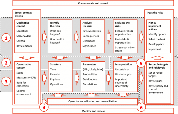
Step 6: Revise the model and its parameters as necessary

The estimate or plan may have to be revised to achieve an outcome required for the project to be a success. In this case, it is good practice to run the model based on the revised plan and estimate to confirm that the changes will deliver the desired outcome and not introduce any new risks.

Project teams will often use these models to explore options and carry out ‘what-if’ analyses, to illustrate to senior managers what challenges a project faces and possibly argue for variations to key performance measures or for additional resources to be allocated to the work.

Summary

Range analysis cannot be a mechanical process, but it should be systematic; Figure 11 shows the six main steps. The diagram highlights what is important at each step – use these to plan the range analysis.

Remember that models are not decision makers. They only help to make sense of a project, and their outcomes must be interpreted for the circumstances and the business requirement in which they are being implemented.