Target construction cost for an alliance contract
Introduction
This case study concerns an alliance established to deliver a major road improvement project. The project involved substantial civil works in addition to the road itself. The alliance included the local roads authority (a Government agency), a large construction company and several smaller technical design and engineering firms.
The description here focuses on the capital cost of the project: an estimate of the uncertainty associated with the estimate of total cost was required, expressed in dollar terms. This was needed to enable a realistic ceiling price to be set for the project for funding purposes, and to develop a target cost for the contract that would:
- Generate effective incentives for all the alliance parties
- Support an appropriate sharing of risks and rewards between them.
Alliances and incentive contracts
Alliances and incentive contracts are intended to share the financial benefits and costs associated with a project between the owner and the contractor, with a particular focus on the project delivery phase. They can be used to focus the attention of the contractor on performance outcomes, as well as limit the cost to the owner. They usually operate under an open-book arrangement between the owner and the principal contractor, and the incentives often cover the capital cost of the project, the completion time, health and safety outcomes during delivery and the quality and performance of the assets created by the project.
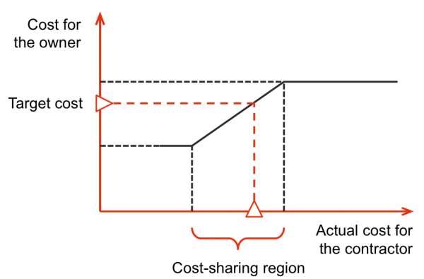
Figure 1 shows the structure of a typical payment approach for capital cost, which is representative of the subject of this case study:
- A designated maximum cost provides a ceiling for the owner, and the contractor would bear any over-runs
- Below a designated minimum cost, the contractor would keep all profits from innovation and efficient delivery
- In the intermediate zone where the actual cost is expected to fall, costs and savings in relation to an agreed target cost would be shared between the owner and the contractor in an agreed ratio.
Figure 1: Cost incentive structure in an alliance
The project cost estimate
The cost estimate for this project was developed in an estimating package that allowed reporting in a variety of forms. It was extracted from the estimating package into an Excel spreadsheet and then simplified to a smaller number of summary items to support the analysis (Figure 2).
Figure 2: Structure of the estimate
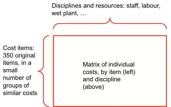
For the analysis, the estimate was structured to show the main cost items – more than 350 of them initially, grouped into a smaller number of items involving similar activities – each with its estimated cost split into individual disciplines or resources:
- Staff
- Labour
- Wet plant (plant plus operators plus maintenance)
- Dry plant (plant only)
- Concrete materials
- Steel materials
- Other materials
- Sub-contracted work
- Other items.
This structure was chosen because many of the sources of uncertainty in the estimate were related to the unit rates for specific disciplines, equipment and materials, and they applied across all of the cost items in much the same way. This simplified the uncertainty model, and it also avoided potential complications associated with correlations. If the costs had been organised into a different structure, some of the common drivers of uncertainty would have affected two or more groups; this would have created complicated correlations between the groups that it is almost impossible to assess and model realistically.
Modelling uncertainty
Sources of risk
Risks in a cost estimate are sources of variation from the base estimate value. They may be positive or negative. They arise from several sources.
- Variations in unit rates are often linked to the time between the development of the estimate and the placing of firm orders and contracts, during which market conditions might change. They tend to apply to all rates in a particular class across the estimate – for example, to all labour components or prices for materials like steel.
- Variations in quantities are often linked to the stage of the design and the completeness of the quantity take-offs on which the estimate is based. They tend to be linked to specific activities or groups of activities – for example, to earthworks estimates or structural design for bridges that may be estimated by different organisations progressing at different speeds. Detailed design is usually not completed before contracts are signed.
- Variations in productivities tend to be associated with the physical environment, like the ground conditions or the weather, proximity to sensitive existing facilities such as homes or transport infrastructure, and to characteristics of the teams doing the work. They tend to be linked to specific kinds of work in particular groups of activities and in particular locations.
- Specific variations may be associated with specific risks that are relevant to particular activities or groups of activities – for example, delays associated with storms and heavy seas when working on foundations and piers in a marine environment, the outcome of detailed investigations such as hydrology studies, or the discovery of unexpected conditions on the construction site such as native heritage artefacts or endangered flora and fauna.
- Global variations may be associated with natural events or specific circumstances that affect most activities in the project – for example, adverse weather or restrictions on site access and operating hours arising from the impact of works on neighbouring communities.
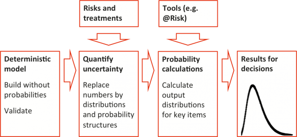
Variations were modelled as distributions and probability structures in the spreadsheet (as described in the following sections) using the add-in package @RISK. @RISK allows simulations to be run and outputs to be obtained in distributional form. Figure 3 illustrates the modelling process schematically.
Figure 3: Model process
Estimating and modelling variations
Most variations took the form of distributions rather than discrete risk events. They were estimated in the form of three-point estimates (B, L, W):
- Best, B, was an estimate of a credible best-case or optimistic outcome
- Likely, L, was an estimate of the most likely outcome
- Worst, W, was an estimate of a credible worst-case or pessimistic outcome.
This approach provided a credible range of outcomes associated with rate, productivity or quantity variations for specific disciplines, resources or items.
Modelling events
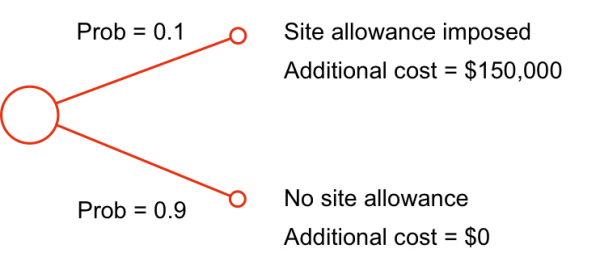
Some risks arose as discrete events. These were modelled as probability trees. For example, Figure 4 shows a simple probability tree associated with the imposition of a site allowance:
- There is a probability of 0.1 that a site allowance will be imposed, which will increase the total labour cost by $150,000, based on an estimate of an additional $1 per hour on labour rates over a total of 150,000 relevant labour hours
- There is a probability of 0.9 (= 1- 0.1) that no site allowance will be imposed, in which case there will be no additional cost.
Figure 4: The site allowance event
In other cases, probability trees with more than two branches were used. For example, when considering storage costs for specialised formwork a three-branch tree was used as a simplified representation of three typical scenarios covering no storage requirement, modest storage needs of three months and extended storage of six months.
Assumptions about uncertainty
Potential variations in the estimate were developed initially by the lead estimator, and discussed and agreed by the wider project planning team, including representatives from all the alliance participants. Some of the assumptions about uncertainty in the project estimate are listed in Table 1 to illustrate the level of detail. The examples in the table also show that, for many items, the value in the estimate was not always treated as the most likely value.
|
Item |
Assumptions |
|---|---|
|
Estimating basis |
The estimate is in today's dollars. Escalation is treated separately. |
|
Staff labour |
The staff labour rate is driven by annual salary increases. The potential rate increase is (0, 3%, 5%). The potential variation in labour hours (excluding schedule effects and so on) is (-5%, 0, +5%). |
|
Wage labour rate |
An enterprise bargaining agreement (EBA) is in place. No change is expected from the estimate in most circumstances, and no savings. The unions might push for a site agreement, which might add $1 per hour to the labour rates (for about 150,000 relevant man-hours of work). The chance of this happening has been discussed with the industrial relations team and management. The initial estimate of the likelihood of a site agreement adding $150,000 to the wage cost is 10%. (Figure 4 shows how this was included in the quantitative model.) |
|
Wet-hire plant rate |
The main driver of variability in wet-hire plant is labour, which may be subject to a different EBA. The estimate is the most likely value; potential range -1% to +5%. |
|
Concrete materials rate |
We may set up a batch plant if quotes for commercial supply indicate this is worthwhile. The estimate is a worst-case value. Assume (-15%, -10%, 0). |
|
Rebar and post-tensioning steel quantity |
This is a design variation. The design is likely to be conservative at this stage of the project. The estimate is the most likely value; potential range -10% to +5%. |
|
Corrosion protection in piers |
It may be a requirement to use stainless steel reinforcing in the piers. This would add cost by increasing both the quantity of steel by about 25% (as stainless rebar is not as strong) and the rate per tonne. This would introduce additional variability, as stainless rebar would have to be sourced from overseas, most likely with a long lead-time, and FX risks would also be introduced. |
|
Earthworks quantity |
Earthworks are not well defined. The estimate is the most likely value; potential range -5% to +20%. This includes all Earthworks items (with Op Code E in the estimate) except those included in Access roads, Items 181-188. |
|
Access road construction quantity |
Work related to access is contained in Items 181-188. The estimate is the most likely value; potential range -5% to +15%. |
|
Geotechnical and rock fall |
Work related to geotechnical matters and protection against rock falls is contained in Items 116-121. The quantity estimate is the most likely value; potential range -5% to +10%. The rate estimate is the most likely value; potential range -20% to +100%. |
|
Access road removal |
Currently there is no provision in the estimate for removal of the access road. It is intended that this will be eroded gradually. Leaving the road may require an environmental impact statement, with associated delays. Removal of the road would incur an additional cost. Currently this would be treated as a contract variation if it were required, to be paid by the owner. No allowance is included in the model. |
|
Schedule variations |
Schedule delay may arise for many reasons. Productivity variability in the main construction items is considered separately, as is schedule variation due to the weather. Items with time-dependent costs include recurring overheads (items 20-58), cranes (86-90) and site general equipment (91-96). The costs for these items are spread over the planned schedule duration to determine an average overhead cost per day. Other schedule variations will affect direct labour and the labour component of wet-hire plant. |
|
Production rates (productivity) |
Productivity is expected to increase as the job progresses. The variation distribution represents an average variation over the construction period. Production variability is driven primarily by wage labour; the production variation should be applied to the labour component of the cost estimate. Additional labour costs are expected to be incurred to maintain the schedule if productivity falls. The estimate is the most likely value; potential range -10% to +20%. Similar distributions are appropriate for each of the three major work areas. There is not expected to be any correlation between these variations, as different crews, in different locations and using different construction methods, undertake the tasks. |
|
Weather variations |
Weather affects direct labour, external dry-hire plant, the labour component of wet-hire plant and project overheads. Based on site and Bureau of Meteorology data, 26 days of rain have been assumed in the schedule. This is the most likely value. In the best case, there might be no rain days, saving 26 days; in the worst case, there might be 60 rain days. |
|
Wind |
Cranes are generally robust in high winds. It is assumed we can work around wind problems by scheduling work and lifts appropriately, or that problem wind days are associated with storms and rain delays, covered under weather variations. |
|
Sea state |
The project may be affected by storms for a period of six months when working on foundations and piers C and D. Time could be lost, and re-work of temporary works may be needed. Assume (1 week, 1 week, 2 weeks). King tides could cause a loss of time if ignored, but it is assumed we can forecast them and program work around them. |
|
Restricted access within the site |
Restricted access within the site, or landslips, could lead to delay. There is a probability of 50% of an incident, with a range of outcomes (0, 1 day, 5 days). |
|
Restricted access to the site |
Restricted access to the site could arise due to a landslip or other incident on the access roads. It is assumed the main effect on the project would be a delay, with direct costs being treated as a variation (if the project must provide temporary bridging or other recovery effort) or borne by the owner. There is a probability of 15% of an incident, with a loss of 20 days. |
Outcomes
The results shown here are based on a version of the estimate normalised to a base value of $100 million. They do not include any contractor's margin, but they do include an allowance for owner’s costs. The estimate was revised progressively as new information became available.
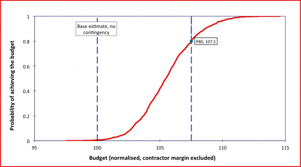
Figure 5 shows the distribution of capital cost. This shows the probability of any particular cost target being achieved by the project – as the target increases, so does the probability that the project outturn cost will be within the target budget. It suited the alliance partners to adopt a conservative view of what could be achieved and so a reasonably high percentile was used to set the cost target. In this case, the 80-percentile value provided a useful target for initial discussions and negotiations. This implied an allowance for risk and contingency of about 7.5% of the initial estimate total.
Figure 5: Estimate variation distribution
Lessons
Alliances and the associated incentive contracts encourage a cooperative and collegial approach to a project. There are incentives for all parties to work together to achieve agreed project outcomes, as the contract structure ensures that everyone benefits from better-than-expected performance. The incentive structure can be adjusted to include many factors of interest to the alliance parties as well as several kinds of targets, for example standard targets relating to ‘acceptable outcomes’ and stretch targets for ‘exceptional outcomes’. Outcomes other than cost are often included, such as the number of safety incidents of various levels of severity or the extent of complaints from neighbouring communities.
The estimate structure for the analysis was relatively simple in this case. It was as detailed as necessary to think about uncertainty in a realistic way and to capture what might happen and what might be important. In general, a simple carefully-designed estimate structure allows more detailed thinking about uncertainty and how it might be managed. Too much detail inhibits this, as people become ‘lost in the weeds’. A structure that is not aligned to the underlying sources of uncertainty generates complicated and confusing interactions that make it difficult or even impossible to create a realistic model.
The P80 value was used as a starting point for the incentive agreement in this case, but any value could be used to start discussions. The full distribution in Figure 5 provides a guide to the upper and lower bounds that might be included in an incentive arrangement like the one illustrated in Figure 1. Clear contractual terms and conditions are still needed to specify what should be included in the incentive arrangement and what might be treated as allowable contractual variations.
- Client:
- Local roads authority (a Government agency), a large construction company and several smaller technical design and engineering firms
- Sector:
- Roads and highways
- Public sector and government business
- Services included:
- Project risk management
- Quantitative modelling
- Cost uncertainty
- Contract support