Some of this material was covered in a PMI webinar in early 2014

The paper is also available here in Spanish. Thanks to Mr Fernando Hernández of Palisade who translated it from the original.

Overview

Methods currently in use to assess project cost contingencies range from flat-rate percentage allowances that would have been familiar to engineers of the 1930s to techniques reliant on computer simulations that have only become generally accessible relatively recently. Some useful modelling techniques that have come to the fore in the past ten years were understood in the 1970s, before computing facilities were widely available or easily accessible, but they could not be adopted widely until computing became cheap and ubiquitous.

In the interim, simpler methods were employed because, in their most basic form, they could be implemented with pencil and paper. As computers became less expensive, more widely available and increasingly powerful, valuable early insights into the nature of project cost uncertainty and how best to analyse it were overlooked by many in the field. Instead of using the power of computers to enable the use of improved methods in this area, early exploitation of rising computer power concentrated on automating the simple manual methods that were already in use and then making them more elaborate. There is a danger that some of these ideas have become so pervasive that users are coming to regard them as standards and fail to recognise that there are better options.

Much discussion in this field is currently framed in terms of the characteristics and features of methods and tools as they compete for attention and commercial prominence. This paper argues that it will be beneficial to focus more attention on the characteristics of the systems being modelled, the projects and their costs, and seek analytical techniques that match them. In particular, the heavy reliance, in some cases exclusive reliance, on representing uncertainty as events is unhelpful. Greater use of alternatives, such as the approach described here as risk factor modelling, and the use of mixed methods will improve the value of cost risk models, reduce the effort required to achieve a realistic assessment and improve understanding of risks and how to manage them.

Introduction

Despite a history going back over forty years, the use of quantitative modelling to set project cost contingencies is not yet a mature discipline. Practices in common use today range from the most rudimentary methods that predate the use of quantitative modelling to ideas that have only come into use in the last decade. Non-specialists are faced with several different and overlapping alternatives, which are often presented as mutually exclusive and in competition with one another. This sense of having to choose between the alternative commercial software packages places the emphasis on the tools, often without reference to the reality they are intended to represent, and sets up a false dilemma for the prospective user.

The legitimacy accorded to some current methods rests on them having been in use for a long time as much as or even more than their objective merit. New risk assessment tools and methods are no doubt prepared in good faith by people who believe what they offer is sound. However, they are sometimes hostage to entrained thinking that has its roots so far in the past that it can appear to be a natural foundation for an analysis simply because it is familiar. It is useful to recall how these entrenched concepts came into being so that we can gain a clear view of their value and understand why they are so prominent despite shortcomings and the existence of superior alternatives.

This paper provides a brief outline of how quantitative cost uncertainty analysis has developed since the 1970s. Much of the argument set out here applies equally well to schedule uncertainty modelling but it is simpler to explain in the context of cost uncertainty. Cost uncertainty is still the major preoccupation of many quantitative risk assessments despite the powerful role of schedule uncertainty in the economic performance of projects.

It is suggested here that:

• A shift in viewpoint away from the present focus on tools and methods towards the characteristics of the uncertainty affecting projects is useful
• That no single type of analysis is likely to meet all projects’ requirements, we need a toolbox of techniques from which to choose
• That some methods in widespread use are a poor fit to the jobs that are pressed into their rigid structures.

This paper builds on material in a recently published book on project risk management (Cooper et al, 2014). It is not intended to provide detailed guidance on any particular method although a brief outline will be provided of the risk factor approach that has proven extremely useful in a wide range of applications as part of a flexible suite of risk modelling methods.

Evolution

Background

A few highlights from the history of quantitative cost risk modelling will illustrate the evolution of the subject and the forces that have shaped it. Parametric techniques (AACE RP 42R-08, 2011), which use data from past projects and the characteristics of new projects to forecast contingency requirements, will not be discussed here in any detail as they are distinct from the class of methods in which uncertainty is expressed in terms of probabilities and probability density functions or distributions.

Even if they have deterministic roots, most cost risk analysis methods, apart from parametric modelling, now use Monte Carlo simulation and they are available to anyone with an ordinary personal computer. Some provide a model structure that is partially predefined, often in the form of a risk data base linked to a table of costs, and some are completely open, such as the many Excel add-in and influence diagram modelling packages on the market.

Current cost risk modelling methods can be grouped loosely into three types:

• Line item ranging, applying a distribution to each line in an estimate or summary of an estimate
• Risk event models, in which uncertainties are described in terms of the likelihood of them arising and the effect they will have on the cost
• Risk factor models, in which uncertainties are described in terms of drivers that might each affect several cost elements and where several drivers might act together on a single cost, with a many-to-many relationship between risks and costs.

History

The most basic approach to setting project contingency allowances is to allocate a fixed percentage of the estimate, perhaps based on past experience or historical outcomes. Some organisations have managed to survive using this approach but it rarely persists once the environment in which they operate changes significantly. As new projects start to diverge from the pattern of past work, this method is likely to fail. It is unable to accommodate fresh sources of uncertainty or a shift in the balance between different sources of risk. Since changes generally introduce novelty and fresh challenges that bring with them additional risk, historical levels of contingency often turn out to be insufficient.

Simple scoring mechanisms have been devised to try to bring more rigour into the assessment of a contingency as a percentage of the base estimate. Some take inputs that rate a project’s scale, complexity, level of definition, use of new technology and other factors on a scale of points, a form of parametric modelling. The tool might recommend a percentage contingency based on a simple sum of the scores associated with all the factors. Scoring methods are usually established within a sector or field that is homogeneous enough to ensure consistency between past and future projects. Even when they have been calibrated to produce a realistic contingency assessment within their bounds of applicability they may struggle when new risks arise.

As computers became increasingly widely available from the 1970s onwards, it became feasible to apply more sophisticated methods to the assessment of project contingencies. Just as a large and complicated cost estimate is broken into smaller, simpler parts so that estimates for the parts can be collected and added to provide an overall estimate, something similar became possible for the uncertainty that a contingency is intended to cover. Models were developed that sought to describe uncertainty in component parts of a project’s cost and aggregate them into an assessment of the overall uncertainty in the estimate.

There are papers describing the use of distributions to represent uncertainty in major projects dating from well before risk models became commonplace. A World Bank publication from 1970 (Pouliquen, 1970), for instance, describes modelling the uncertainty in economic forecasts of infrastructure projects, including costs and benefits. An indication of the challenges these pioneers faced is their report of taking six months to develop a program to evaluate the first model and two months for the second one even though it reused some of the code from the first one.

The World Bank models used relatively few uncertainty factors and yet the team confined the simulation runs to evaluate their models to three hundred iterations. It is not clear if the cost of computer run time was an important consideration but it was significant enough to be mentioned. The paper discusses costs for both developing the code and running the models.

At this time, apart from financial and other business systems, computing facilities were generally confined to specialist units within large organisations, a few university departments and research institutions. Not many businesses used a computer for technical modelling. In this environment, few organisations were in a position to follow the path taken by the World Bank. Even those engineers who had access to computers and wanted to explore the subject found that realistic models often stretched the capacity of the available machines. Software had to make careful use of RAM measured in kilobytes, programs were coded on punched cards and submitted for batch processing with a turnaround counted in days, and most installations rationed access to the CPU as well as limiting maximum run times.

Innovative responses to these limitations were developed to meet particular modelling requirements. Chapman and Cooper described an ingenious numerical integration technique, developed by Chapman in work he was doing for BP on North Sea projects. The controlled interval and memory (CIM) (Chapman and Cooper, 1983) method was designed specifically to facilitate project risk modelling within the limitations of the memory and processing power available at the time. Applications are described in the book by the same authors (Cooper and Chapman, 1987). The book illustrates the extent to which the use of quantitative analysis was influenced by the capacity of the computing systems available at the time.

Simple quantitative methods

At about the same time as these early cost risk modelling exercises were underway, from the 1970s onwards, project management gained popularity as a means of building and developing assets and projects became increasingly complicated. The need to provide realistic cost contingencies became more and more pressing. Ironically, some of the most challenging projects involved computing and related systems, the technology that would later make it easier to model project cost uncertainty.

Major infrastructure and engineering projects presented similar challenges, increasing scale and complexity resulting in rising levels of risk. Specialists were able to assist major projects (Cooper and Chapman, 1987) but many projects did not have access to these services and many more would not even have known that they existed. The rate at which computers eventually came to be used to support projects was dictated by increasing supply, the availability of computing power, at least as much as by increasing demand, the growing scale and complexity of projects.

The author’s experience in the ICT sector at this time was that each new medium to large scale project seemed to throw up risks that had not been encountered before and all concerned struggled to know how to make financial provision for the uncertainty they represented. There was a clear need for a better way to assess contingencies and to understand the risks that made them necessary so that those risks could be controlled.

With more subtle techniques confined to specialists who had access to general purpose computers and people to program them, simple methods of assessing contingencies were sought. For a long time, a risk had been synonymous, in common usage, with an undesirable event. An approach based on risk events, illustrated in Figure 1, was widely employed to assess project contingency requirements. Each risk is described by a probability of it happening and the cost impact it will have if it does happen. The expected value of the risk is the product of these two parameters. It is simple, it can be carried out with pen and paper, and it satisfies the desire to see risks as events. Unfortunately, many sources of uncertainty cannot be described well using just a probability and an impact in this way.

Figure 1: Contingency calculation for risk events

To see why this structure presents problems, consider a simple example. It might be clear that the cost of office accommodation for a project team could differ from the value assumed in the team’s estimate but it is difficult to capture in an event the fact that the variation might be positive or negative or the fact that the variation might be small or large and the larger the variation, the less likely it is to occur. The possibility of positive as well as negative variations was sometimes addressed by introducing opportunities, a word chosen to mean the opposite of a so called negative risk. Opportunities were represented as events with a probability of occurrence and an impact that represented a cost saving or income.

Despite being a poor fit to many project uncertainties, the general view that risks are undesirable events and the difficulty of using more sophisticated modelling structures without a computer left many people unaware that there was an alternative. These simple methods appear to give an expected value of risk and can be implemented with pen, paper and a calculator. They became established and were assumed to be sound simply because many users never saw anything else. As computers became more widely available, the simple pen and paper methods were automated and so gained even greater credibility.

Monte Carlo simulation and simplistic applications

Inexpensive Monte Carlo simulation software became available for personal computers in the early 1980s. The software made it possible to represent uncertainty in quantitative models and evaluate the aggregate effect of multiple uncertainties.

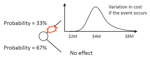
Some practitioners used this new capability to elaborate on existing methods. In particular, the risk event approach depicted in Figure 1 was extended by describing the impact of a risk as a distribution of outcomes instead of a fixed value, as illustrated in Figure 2. This lent the method additional weight as it then appeared, and still does to some, to be very sophisticated. The addition of distributions to describe impacts did nothing to alter the fact that while some risks and their effects are well represented as events many are not. The simple example given earlier, office space that might cost more or less than has been assumed, can be pressed into the event form by assigning it a 100% chance of happening and making its minimum negative but it is not really an event. Adopting this approach interferes with clear thinking about more complicated risks.

Figure 2: Risk event with distributed range of outcomes

The emergence of the risk register as the focus of project risk management at about the same time, the 1980s, saw risk registers being combined with Monte Carlo simulations using a probability and impact distribution to model each risk register item. The resulting tools are superficially compelling because they match the common view that risks are events and they offer support for project risk register maintenance, which is a necessary function but more properly concerned with risk treatment and control assurance rather than contingency assessment. Tools using this structure seem like a natural starting point for thinking about risk. There is further appeal in having a risk register and quantitative model housed within a single package (although co-existence does not always guarantee integration).

The second simplistic application of Monte Carlo simulation is an extension of the practice of engineering estimators to assess a contingency value for each line in their estimate then add them up to get an overall contingency figure. Instead of assigning a single figure to each line, this technique, often described as line item ranging, assigns a range of costs or a range of percentage variations around the base cost estimate, uses those to define a distribution of variation in the cost and uses Monte Carlo simulation to assess their aggregate value. Just as placing a distribution on the impacts of events was an easy extension of the risk event model, placing a distribution on the costs of items in an estimate was an easy extension of standard estimating practices.

The line item approach is generally not recommended for any but the simplest high level estimates. It might be sufficient for an order of magnitude estimate with only a handful of lines, or a simple part of a larger estimate, so long as the cost item uncertainties are independent of one another. For anything beyond this, experience shows that it almost invariably fails to provide a realistic assessment of contingency requirements and this is borne out by research published by IPA (Juntima and Burroughs, 2004).

Line item ranging will typically produce a narrow range of possible costs, giving a false sense of confidence in the outcome, and understate the contingency required especially if this is set to provide a high level of confidence in the adequacy of funding allocation, say the P90 level. This is primarily due to the fact that sources of uncertainty often each affect several costs and simplistic models fail to take this into account.

Many costs have similar drivers of uncertainty. Uncertainty in labour productivity, for instance, will cut across most of a project’s labour costs and also affect the amount of associated facilities or plant the project will require. Uncertainty in these costs will be correlated. Attempts to use correlations in a model to represent this effect can, in theory, produce plausible contingency forecasts. However in reality, with large numbers of cost items to consider, realistic correlation modelling in project cost risk analysis is rarely practicable. Most people are unable to make realistic estimates of the amount of correlation to expect between two or more costs affected by the same sources of uncertainty.

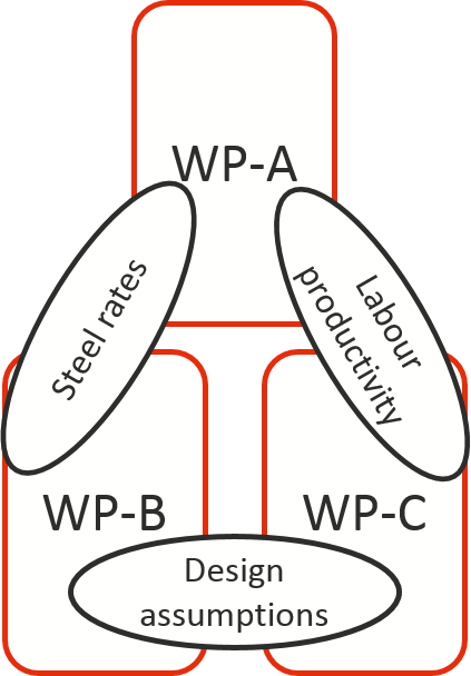
Figure 3 illustrates a situation in which three work packages of an engineering project (WP-A, WP-B and WP-C) might be subject to three sources of risk that link the uncertainty in the three costs. Not only is it challenging to assess each level of correlation in isolation but the three correlation factors have to obey mathematical constraints that bind them together, which will rarely be understood by those who have to assess the values of the correlation factors.

Figure 3: Overlapping correlations

Correlations in a model can be adjusted until the output meets expectations, so called back fitting, but this rarely yields any justification for the correlation values used or insight into the factors causing the correlation. In these situations, the relationship between the model and the real world is either tenuous or heavily obscured.

Some authors have recommended the use of a standard level of correlation between a project’s cost distributions (Smart, 2013). While this may prove a useful administrative approach for contingency allocation within a body of projects having broadly similar characteristics, such an assumption is unlikely to be realistic if the structure and characteristics of the costs in future projects differ from those used to infer the standard levels of correlation. It also provides little or no insight into the nature and source of the uncertainty affecting the cost and so is unlikely to generate support for conclusions drawn from such a model, let alone assist efforts to control the risks. AACE International recommends that the line item approach be avoided (Hollmann, 2009). Research published by IPA (Juntima and Burroughs, 2004), in which this simplistic application of Monte Carlo simulation is described as risk analysis (a term now taken to have a wider meaning) describes the method as “a disaster” especially where project definition might be incomplete when they say the method is “inconsistent and unpredictable”.

Risk event models

Much current practice consists of methods with their roots in a past era. Methods are still in use that were once attractive because they could be carried out with pen and paper. They may have evolved into more elaborate looking computerised versions but they are still as limited as they ever were. In particular, models based on risk events, bolstered by an association with risk registers, have become deeply entrenched in tools and methods that are in widespread use. It is useful to consider what risk event models can and cannot do.

Some projects proceed with significant discrete risks in play. A large industrial plant might be designed anticipating specific environmental legislation. The fall back position may be to modify the plant and use an alternative process, generally less productive or more costly. IT and communications projects might be implemented in the expectation that a supplier’s promise to provide a key software component will be fulfilled. The team might know that, at some additional cost, an in-house development can satisfy the requirement if the supplier fails to deliver.

Most large projects face few really large discrete risks with a significant chance of happening. Project owners demand that exposures to large step changes in their costs be designed out, as far as it is possible, before they sanction the investment. If a large investment is undertaken despite such a risk, that risk will usually be addressed as a separate management task. Separate funding, risk treatment actions and responsibilities will be put in place to deal with it rather than allowing one major concern to skew the management of the general contingency.

Where really large event risks could arise and are to be included in the contingency, a discrete risk model is realistic and is recommended for that part of the cost uncertainty. If there are a few discrete risks that are independent of one another, or if the model is elaborated to embody any interdependence in a realistic fashion, this should be straightforward. However, problems can arise when event models are used to represent a multitude of smaller risks that might overlap or interact, such as all the items in a large risk register, or where they are used to represent risks that are difficult to frame as events because they are naturally seen as continuous variations around the values assumed in the base estimate not as events.

To see why discrete risk representation is ineffective where there are many factors contributing to cost uncertainty, consider what might affect the number of hours effort that will be expended to complete a project. Uncertainty about weather conditions and labour productivity arises in many construction projects. The weather will generally have some potential to be better and some potential to be worse than assumed in the estimate, and outcomes in between the best and worst possibilities could all occur with a declining likelihood towards each extreme. As with the weather risk, the probability that labour productivity will differ from the estimate is almost certain and the defining characteristic of this uncertainty is a distribution of outcomes rather than an event, a distribution that might affect several costs. The discrete nature of a risk event bears little relation to the continuous nature of these and many other uncertainties.

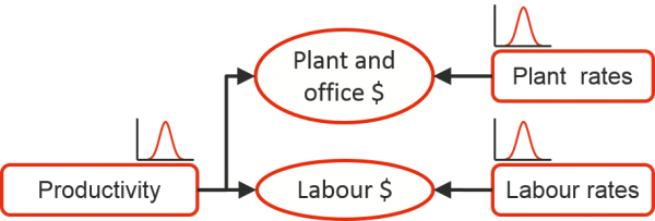
A second problem is that interactions between uncertainties are all but inevitable in real projects. For instance, risks causing variation in the total number of labour hours required by the project, such as productivity uncertainty, will interact with risks that could affect the unit cost of labour, labour rate uncertainty. Their combined effect can exceed the sum of their two effects in isolation. The interactions between three common sources of uncertainty in a construction project are illustrated in Figure 4, which represents just a fragment of a complete model. Both cost items, labour cost and plant cost, are subject to two sources of uncertainty; uncertainty about productivity that affects both of them, and uncertainty about the rates for labour and plant, the cost per hour in each case. In each case, the combined effect of the two uncertainties will exceed the sum of their separate effects. It is clear that these effects cannot be isolated from one another nor can they be combined realistically into a single source of uncertainty.

Figure 4: Interactions between uncertainties

A further challenge is that risk events’ impacts might overlap, especially where those impacts arise from their effects on the duration of tasks. If there are two or more delays to the one task, such as interruptions caused by inclement weather and separate interruptions due to industrial action, their impacts will rarely fall exactly in parallel or exactly in series. As the number of risk events defined for a project rises, the number of possible interactions and overlaps grows at a combinatorial rate and it is quite likely that at least some of the possible associations will be overlooked in a model even if the tool permits them to be represented.

Risk events are a necessary part of the modelling toolbox but they are ill suited to representing many of the uncertainties affecting most project estimates. Alternatively, the aggregate behaviour of a large number of possible events can be described as a continuous range of outcomes in factors driving the cost, and this is the basis of risk factor modelling. Risk factor modelling is closely related to the approach described in the AACE International recommended practice on range estimating (AACE RP 41R-08, 2011).

Risk factors

As Monte Carlo simulation capability became available on standard personal computers, some in this field rediscovered or reinvented the approach adopted by the World Bank (Pouliquen, 1970), in the 1970s. When the World Bank team embarked on this analysis for the first time, with no precedents to cloud their thinking, they concluded that it is better to focus on sources of uncertainty than on individual cost items as a line item approach would do. They realised that correlation is a problem with line item ranging and, although it is a secondary matter, it is of interest to note that they found that the precise shapes of the distributions used to describe uncertain values are not as important as people think. In this context, as the authors said, a risk analysis

does not aim to give the exact true distribution we would obtain if we were omniscient but one that represents the judgement of an appraisal team

These conclusions are now regarded as marks of good practice, but good practice is not always common practice.

Risk events represent a bottom up approach to understanding uncertainty. By contrast, the situation represented in Figure 4 and similar more complicated interacting uncertainties can be modelled realistically, with little difficulty, using risk factors. This is a top down approach that capitalises on the judgement of experienced project and subject matter experts to assess the range of uncertainty a project might face using a model to integrate the process.

Risk factors represent cost drivers that are subject to uncertainty. They are often closely aligned with key estimating assumptions such as labour productivity or the duration of a project. A useful set of risk drivers will be a good fit to the cost and also a good fit to the major sources of risk, bridging the two sets of project information. It is a way of mapping the relationship between the multitude of uncertainties affecting a project’s cost and the cost itself.

As was pointed out earlier, risks interact and their effects overlap. Risk factor models can accommodate this because one risk factor can represent the effect of more than one of the risks in the register and one risk’s effects might show up in more than one risk factor. Each risk factor may then in turn be a driver of more than one part of the cost and one part of the cost may be driven by more than one risk factor.

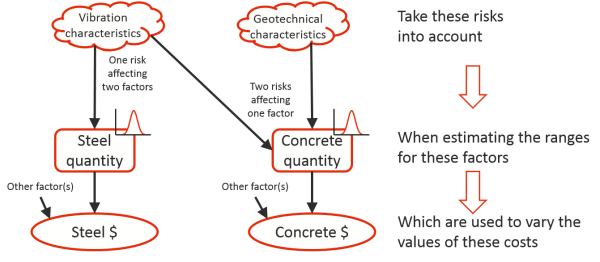
For instance, as illustrated in Figure 5, uncertainty about the size and vibration characteristics of a large machine, a single risk, could contribute to uncertainty about the quantity of concrete and the quantity of steel required for a platform on which it will be mounted within an engineering plant, two risk factors affected by the same risk. At the same time, the quantity of concrete may also be subject to uncertainty about the geotechnical characteristics of the earth below the platform so the one risk factor is subject to, at least, two risks.

Figure 5: Examples of risk and risk factors driving costs in an engineering project

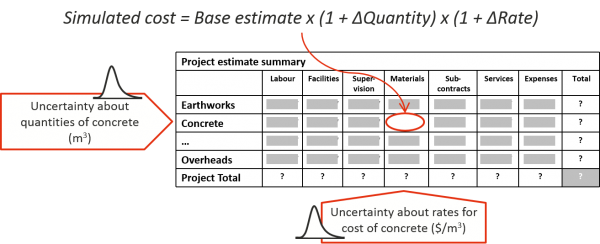
More than one risk factor is then often linked to one piece of the cost as happens when there is uncertainty in both the quantity of a bulk material required and the unit cost of the material, which is illustrated in Figure 6. To arrive at an efficient model, it may be beneficial to group some costs together and split others up. For instance, the cost of temporary facilities for a project team might include some fixed elements and some that are sensitive to how long the project will take to complete. Breaking out the time dependent part will allow uncertainty about the duration to be applied to that part of the cost.

Figure 6: Risk factor modelling

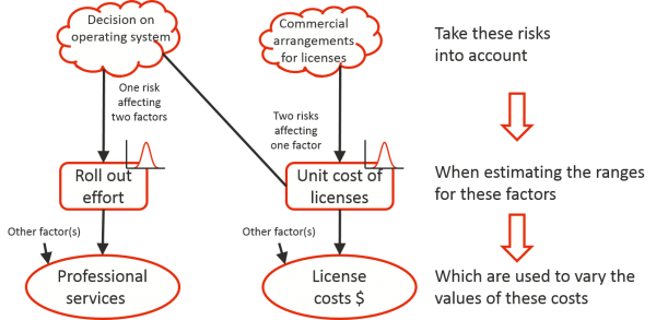
This approach works well in other sectors as well. In the IT sector, a similar situation could arise with the cost of user training for a system roll out, as illustrated in Figure 7. Uncertainty about a policy decision, to be taken at a senior level outside the project, on whether to roll the system out on the users’ existing desktop operating system or upgrade the operating system at the same time will affect the cost of licenses and the amount of effort required for the roll out, two factors affected by the same risk. At the same time, uncertainty about the commercial arrangements under which the licenses will be purchased will also affect the unit cost of licenses so the one risk factor is subject to, at least, two risks and once again any part of the cost might be affected by two or more risk factors.

Figure 7: Examples of risk and risk factors driving costs in an ICT project

While a risk register might have a large number of entries, twenty to thirty risk factors is usually all that is required to describe possible variations of a project’s real cost from the initial estimate and wrap up the effects of the individual risks. Curran reports finding that, of several hundred projects that were examined, more than ninety percent required no more than thirty factors to represent cost uncertainty (Curran, 1989). The growing body of experience with risk factor models bears out this observation.

One way to understand the efficiency and realism of a risk factor approach and its relationship to risk events is to observe that a multitude of discrete events can usually be found within what we perceive as a continuous variation. For instance, many events could affect labour productivity yet we can understand their net effect without needing to isolate and describe each single event.

As a very small illustration of this, documents required to carry out a particular task might be provided late, resulting in personnel wasting time as they organise themselves to tackle work they had intended to do later. The same documents might be delivered on time but perhaps incorporate errors meaning that tasks are completed incorrectly and have to be reworked. An individual worker might be part way through a task when they are taken ill and leave before they can document their progress making it difficult for someone else to pick it up. Those are just three events that might or might not happen and within a real task of a reasonable size they could each happen more than once, especially the first two. It is possible to imagine an almost unlimited number of similar events at work within a single cost risk driver such as uncertainty in labour productivity.

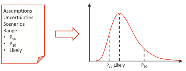
Assessing the aggregate effect of all these small events as a range is relatively straightforward. It results in a clean model with a clear connection from the way subject matter and project specialists think about uncertainty and describe it, to the model itself, and then to the outputs it generates. A risk factor is usually described with a three-point estimate that is used to define a probability density function that represents that factor in a model, as illustrated in Figure 8. A lot of attention is often given to the shape of the distribution but, within reasonable bounds, so long as the three key values shown here are preserved, the choice of distribution type has little effect on the outcome.

Figure 8: Describing the range of a risk factor

Since one source of uncertainty might influence two or more risk factors, the possibility of correlation between risk factor distributions should be considered. Where there are many individual risks at work, as described for the example of labour productivity, unless two factors share a large number of underlying uncertainties, strong correlations between factors are not common and this is usually apparent to those assessing the ranges. In fact, the exercise of identifying drivers for the model, the risk factors, generally seems to result in factors that are fairly independent of one another.

Correlation between risk factors may arise in intangible or complex underlying drivers such as the state of the economy. A risk register might, for instance, include reference to a general rise in economic activity driving up costs or a softening of the economy yielding some savings. Economic modelling is beyond the competence of most project teams and a notoriously complicated matter in its own right. However, the state of the economy might be considered in the assessment of ranges around assumed bulk material and labour rates and around assumed levels of labour productivity where high levels of economic activity make it difficult to attract the best personnel and productivity might suffer.

Where there are several risk factors that are subject to general economic conditions, the implications of these being correlated may be examined as a ‘what-if’ analysis, testing the effect of there being none or being 100% correlation between them. This can be discussed with the project team to determine whether market based correlation should be included or not.

The common understanding of risks as discrete events is not entirely unrealistic but it has limited value beyond dealing with a relatively small number of large risks. It is more realistic, more informative and more cost-effective to represent most project uncertainties in terms of carefully chosen risk factors that encapsulate the myriad of small events that could arise during a project’s execution while preserving important separations and allowing for important interactions that exist in the real world. Individual statements of risk are central to identifying where to put effort and other resources into enhancing a project’s chances of success but this is a different role to that of assessing the overall contingency.

Coherence between real world uncertainties, the expert judgements of those who describe them, the models based on those judgements, and decisions based on the models is readily achieved by this means. This analytical process, which is more than just a model, generates valuable insights for risk management, not just a mechanistic assessment of a contingency figure in isolation. A risk factor model may be augmented with additional components such as a few large events or other special features, but experience shows that the bulk of the uncertainties in infrastructure, resources, engineering, ICT and organisational change projects are readily and realistically addressed in terms of risk factors.

Current practices

Practices in use today include everything from methods that arose before models started to be employed, flat rate contingency percentages, through to some that have only become established recently despite having been foreshadowed decades ago. In the absence of a consensus among specialists, there is no convergence on any particular approach in the wider community of analysts.

Many organisations see quantitative risk analysis as a problem. They struggle to gather sufficient expertise in-house to address the subject themselves and quite often, failing to understand the value it can deliver or the implications of getting it wrong, are unwilling to engage external advisers. Where organisations are trying to improve contingency assessment it is often due to one or more major projects going a long way over budget or a pattern of consistent smaller scale cost over-runs becoming too big to ignore.

There is a clear trend towards methods and tools that purport to reduce the users’ need to investigate risks for themselves. Some of these are attractive to project organisations as they appear to enable contingency requirements to be assessed with limited specialist expertise. Users may be attracted by the promise of being able to rely on the credentials of a commercial tool to limit both scrutiny of their conclusions and the demand for new skills.

There is no reference body or standard that commands the full support of the majority of specialists working in this field. Guides produced by the major project management organisations rarely figure in professional discussion about cost risk modelling. They are, by their very nature, compromise positions struck among a diverse group of people so they tend to lag behind developments among the leading professionals. In addition, the methods used by these leaders are still evolving so that it is very unlikely that any de facto standard, let alone a formal standard, will emerge in the near future.

The most authoritative guidance that does appear to command widespread respect, if not complete adherence, is the set of recommended practices published by AACE International. These cover several methods that are recommended for modelling cost uncertainty including range estimating (Curran, M.W. 1989), which is similar to the risk factor approach outlined here. They also recommend that the widely used method known as line item ranging be avoided (Hollmann, J.K. 2009).

The international standards ISO 31000:2009, Risk Management, and IEC 62198:2013, Managing Risk in Projects – Application Guidelines, provide guidance on risk management in general and for projects respectively. They adopt a view of risk that places events, positive or negative, within a broader concept that includes other forms of uncertainty affecting the achievement of objectives. This is consistent with modelling uncertainty in large and complex projects, using risk events as just one of the mechanisms required to produce a realistic representation of cost risk, with risk factors being used to model the bulk of common project cost uncertainty.

Conclusions

Practices that grew out of a need to deal with project cost uncertainty in a time when the power and availability of computers were, by today’s standards, very limited have become entrenched in common usage long after the constraints that led to them being adopted have disappeared. A preoccupation with risks as events and with a tabular risk register as the core of a risk management process have seen these methods formalised in tools and guidelines for decades to the point where many users are unaware that there are better options. Similarly, the simplistic approach known as line item ranging has been widely taken up just because it is very simple and, despite its serious shortcomings, has become so familiar that many users never question its merit.

There has never been a greater selection of computer-based tools to support cost risk assessment. Reviewing them all would be a large task in itself but, in light of the points made earlier, it is useful to note that some embody a structure that presumes all risks can be described within one fixed framework, generally based on a risk event structure, often associated with a risk register, or the simple tabular form of line item ranging. Others provide a framework with flexibility to choose from a selection of building blocks and configure the way they interact, while some are almost completely open and allow modellers freedom to create any structure they feel a project requires.

Where major events can affect a project, using an event structure for modelling those events is clearly appropriate but it is not generally suitable to model all the uncertainty in a project. Where uncertainties are more naturally characterised as continuous variations, an alternative approach is to be preferred and the risk factor method is often a good fit. A risk factor approach augmented to include any really significant risk events has been shown to assist in understanding project risk as well as in assessing contingency requirements. The inputs are easily understood and the exploration of cost drivers is of benefit to management as well as allowing a realistic assessment of possible cost outcomes. Line item ranging is generally to be avoided apart from possibly using it for small parts of an estimate subject to straightforward uncertainties that are independent of one another and the rest of the cost.

Each project should be modelled in terms that match its particular characteristics. Seeking to force a project’s uncertainty into a predefined structure is poor practice. It might not always be possible to model every aspect of a project’s uncertainty entirely faithfully, but better outcomes will always be achieved if reality is considered first and the model follows it, rather than having the analysis dictated by the fixed characteristics of a predefined model or tool.

References

AACE International (2011) Recommended Practices, RP 41R-08: Risk Analysis and Contingency Determination Using Range Estimating, AACE International, Morgantown WV

AACE International (2011) Recommended Practices, RP 42R-08: Risk Analysis and Contingency determinations Using Parametric Estimating, AACE International, Morgantown WV

Chapman, C.B. and D.F. Cooper (1983) Risk engineering: basic controlled interval and memory models, J. Opl Res Soc, 34(1), 51-60

Cooper, D.F. and C.B. Chapman (1987) Risk Analysis for Large Projects. John Wiley, Chichester

Cooper, D.F., P.M. Bosnich, S.J. Grey, G. Purdy, G.A. Raymond, P.R. Walker and M.J. Wood (2014) Project Risk Management Guidelines: Managing Risk with ISO 31000 and IEC 62198. Second edition, John Wiley, Chichester, 2014

Curran, M.W. (1989) Cost Engineering, Range Estimating: Measuring Uncertainty and Reasoning with Risk, 31(3), 18-26, AACE International, Morgantown, WV

Juntima, Gob and S.E. Burroughs (2004) AACE International Transactions, Exploring Techniques for Contingency Setting

Hollmann, J.K. (2009) AACE International Transactions, Recommended Practices for Risk Analysis and Cost Contingency Estimating, AACE International, Morgantown, WV

Pouliquen, L.Y. (1970) Risk Analysis in Project Appraisal, World Bank Staff Occasional Papers, No. 11, Johns Hopkins Press, Baltimore

Smart, C. (2013) Presentation to ICEAA, Robust Default Correlation for Cost Risk Analysis