Summary

This case study outlines how a property development company analysed uncertainty as an input to a Board decision. It discusses practical ways to simplify the structure of property development models to include uncertainty estimates in a reasonable way, to overcome problems associated with the inherent complexity of many of them. It also notes the importance of setting workshop agendas to make it easy for senior executives to participate.

Background

The development opportunity

Our client, a listed property development and management company, was examining a development opportunity that arose as part of a government-sponsored urban refreshment. The development site was centrally located in an area with significant potential for population growth and commercial expansion. Part of the attractiveness of the opportunity was the absence of competitive centres of the kind in which the company specialised, so there was likely to be an important ‘first mover’ advantage if the opportunity could be realised.

The company had compiled a rich database of quantitative research, based on analyses of the retail, commercial and residential market, identification and analysis of competing centres, telephone surveys, community consultations, and a variety of benchmarking activities. It had concluded that there were powerful fundamental reasons for examining the opportunity in detail.

It prepared an extensive set of development options, with initial assessments of the main strategic and commercial opportunities and threats, and initial financial analyses. It had selected a preferred option from this set for detailed analysis and modelling. The preferred option was a mixed-use development with retail, commercial and residential components, outlined in Table 1.

Purpose of the analysis

The objectives of the modelling and analysis in this case were to:

• Help to identify and manage the main drivers of uncertainty in the financial outcomes of the development
• Present information to the Board to assist in the approval process for the next phase of the investment
• Demonstrate how the company’s modelling process could be simplified and generalised for easier application to other development decisions.

The company’s investment modelling

The company used spreadsheet models routinely for examining its investments and managing its assets. Some years before this case study, it started to use @RISK as a tool for exploring some of the uncertainties in the developments and large projects in which it was engaged. However, the models it was using were relatively large and not readily amenable to being generalised to other projects.

The company now wanted to reinvigorate the way it examined uncertainty in its investments. This had several implications for the modelling activity outlined here.

• This development was to be be used as an example investment. Ideally, the model prepared for it would be simple enough to be adaptable to other similar projects.
• The model would be relevant to the early stages of a potential investment when strategic decisions were to be made. In particular, it should assist in identifying the main drivers of uncertainty and their effects, and produce outcomes that could be adapted for presentation to the Board.
• @RISK was the tool of choice for modelling uncertainty.
• While the quantitative model for this development would be prepared by a small team within the company, it should form the basis for training a wider group of business analysts.

Quantitative analysis

The quantitative analysis

This case study describes a quantitative risk analysis of the cash flow of the development opportunity. The assessment included:

• Preparing a high-level quantitative model of the development, to examine the overall financial value of the centre and the uncertainty in this value
• Conducting workshops to discuss and quantify the main drivers of uncertainty in the value of the centre
• Reviewing, discussing and revising the quantitative model and its results.

The model

Quantitative analysis of the kind used in this case begins with a financial model of the development. Here it drew on information from an existing financial model built in Excel. The structure of the model was simplified for the risk analysis to make it easier to focus on uncertainty. The simplified structure was similar to the overview cash flow presentation that was used routinely to brief senior management and the Board.

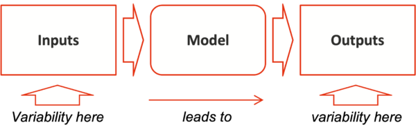
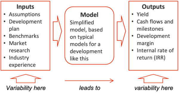
Uncertainty in the inputs to the model was examined, and specific potential variations were represented in the form of probability distributions. These distributions were combined using Monte Carlo simulation with the package @RISK, to generate distributions of the model outputs that were most important for decisions. The structure is summarised in Figure 1.

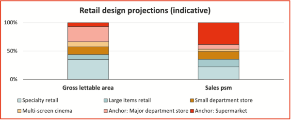
Six categories of retail tenants were modelled. Figure 2 shows the relative projections for gross lettable area allocated to each category in the initial development design, the initial estimated sales per square metre of lettable area for each, and the initial base rent.

• Gross lettable areas were treated as fixed design parameters for the main development option as these are choices the client can make, not uncertain or risky values.
• Sales per square metre (psm) and sales growth were estimated initially from company data, adjusted for the specific site. They were represented by distributions in the quantitative model.
• The initial base rents were estimated from analyses of comparable rents nearby. Contractual arrangements were already in place for the cinema and the two anchor tenants, so their base rents were fixed in the model; base rents for the other categories were again represented by distributions.

Senior executives with responsibilities for the development decision participated in workshops to discuss the main drivers of variability in the financial outcomes for the development and to estimate ranges used to define distributions for them in the model. During the workshop, each item in the model structure was addressed. The main assumptions, sources of variation, and high, low and likely scenarios were discussed, and values associated with each of the scenarios were assessed.

Detailed notes on the discussions were recorded in data tables similar to the template in Table 2. Tables like this make the assumptions explicit, so they can be examined and tested and the estimates can be adjusted if assumptions change. The tables also provide a convenient means of explaining risks to other people.

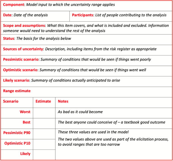
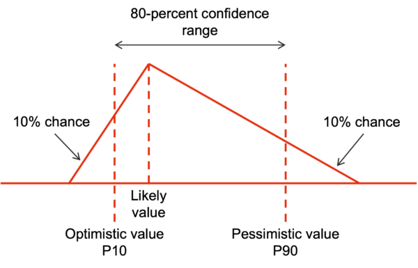
The values for the high, low and likely scenarios (the lower three lines in the table), were interpreted as 90th-percentile, 10th-percentile and most likely values for triangular distributions of the form shown in Figure 3.

Correlations in the model

Correlation between separate uncertain values or distributions must be represented in the model when combining distributions. If it is not, the outcome distributions tend to be narrower than can be expected in reality and the overall variation may be understated, creating a false sense of security.

However, the extent of these correlations is often difficult to estimate, so where possible, we try to identify drivers of variation that affect more than one part of the estimate. We represent the drivers in the model and estimate them explicitly so that we can include their effects on other parts of the estimate arithmetically in the model. We adopted this approach for global economic parameters like inflation.

For example, construction cost variability was estimated as an additional variable margin on top of the inflation rate. The margin variation estimate took account of regional infrastructure projects, which would affect the local prices of concrete and steel, and commercial and education projects, which would affect fit-out cost rates.

Variations in the initial sales per square metre were likely to be driven to some extent by economic, demographic and market conditions in the region and the perceived attractiveness of the centre. Sales growth was likely to be subject to the same set of influences. It was not possible to fully isolate a common driver, so a correlation matrix was used in the model to link the variation in one of these factors to the variation in the others.

A conservative approach was taken with the correlation coefficients, setting them to 100% for the relationships between all tenant categories. This implied that the initial sales and sales growth for most categories would rise or fall together according to the characteristics of the local catchment. There would be no opportunity for a fall in one part of the cash flow to be offset by a rise in another, as might happen if they were independent of one another.

A similar approach was taken for base rents, where the availability of quality retail and commercial space nearby would tend to drive all rents up or down together. A high degree of correlation was assumed for all categories except the anchor tenants, a large supermarket and a leading department store, for which lease arrangements had been completed already.

Initial operating expense variability was judged likely to be driven by general inflationary and other pressures, with labour and utilities costs being two of the more obvious explicit drivers. Again, a high level of correlation between these costs was assumed initially, a conservative assumption.

Table 3 summarises the correlations included in the model.

Model outcomes

The quantitative model generated distributions for development characteristics the Board needed for its investment approval decision. These related to yields in the first year of operation of the centre, 10-year returns for the centre, and development margins. They were calculated for the retail component alone, for the combined retail and commercial component, and for the development as a whole.

As an example, Figure 4 shows the distribution of returns over the first 10 years of operation of the centre. It covered the retail and commercial components, the two areas the company intended to manage over the long term.

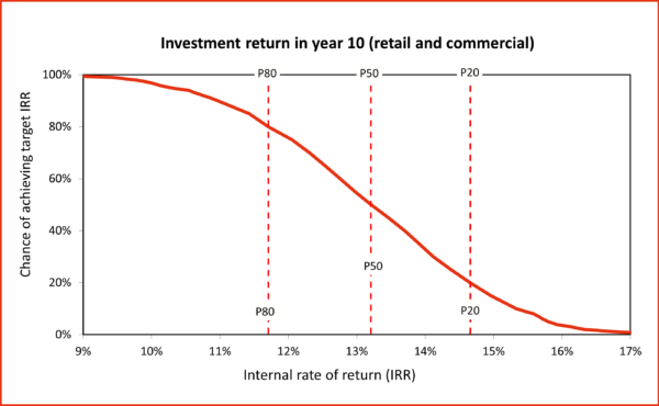
Figure 5 indicates that the main drivers of uncertainty in the return (represented by the width of the horizontal axis in Figure 4) are uncertainties in the gross rents per square metre. The uncertainties in the specialty retail and commercial rents are the most significant drivers, followed by the uncertainty in small department store rents. (Remember that base rents for the anchor tenants had been negotiated already, so there was no variability associated with them in the model.)

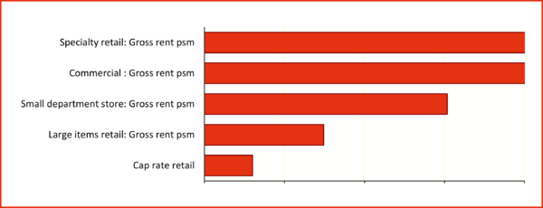
Figure 6 shows the variability in the opening date for the centre. Dates have been adjusted for confidentiality. The jagged line is an artefact of the month-based timetable in the preliminary schedule included in the model. The company intended to conduct a more detailed schedule analysis in the next phase, after Board approval; this level of detail was suitable for the immediate decisions that were needed. In particular, the drivers of the variability in the schedule, shown in Figure 7, were not expected to change, and they reinforced the importance of approval processes. Approvals were already a major concern of the Board.

These and related financial and schedule analyses allowed the Board to include the uncertainty surrounding the forecast outcomes of the project in their decision making.

Complexity in development models

Levels of detail in models

Models for the financial evaluation of property development proposals often have a high level of detail. For example, specialty retail was grouped into one category in the quantitative model used in this case, but development models usually consider the characteristics of specific classes of retail, and sometimes retail is disaggregated to the level of individual stores. The reason for this detail is that financial models are used for far more than financial evaluation: they are comprehensive models that form a base for development planning, operations planning and marketing as well.

A high level of detail is rarely helpful when modelling uncertainty. Several problems arise if a quantitative model attempts to represent many minor items individually. The multitude of minor items usually include groups that will all behave in the same way as values vary, i.e., they are correlated.

As discussed earlier and noted in Table 3, there are many factors that drive elements of a development model in similar ways, such as sales volume and growth, net rents across categories and operating expenses. Ignoring this correlation is not a realistic option: combining many distributions with the assumption that they are independent when in fact they are not means that, during a simulation, high values of one will cancel out low values of another when in reality this will not happen.

Estimating the correlation between each pair of distributions is not practicable either: there is rarely enough useful and relevant data to calculate reliable correlation coefficients; few people understand correlation sufficiently to estimate coefficients well, and there are mathematical relationships that constrain coefficient estimates when more than two variables are correlated together. Modelling the drivers of correlation explicitly is only possible if the relationships are well-enough understood to develop arithmetic representations of them, and if the drivers themselves can be estimated reliably, something that is rarely possible.

As well as these modelling factors, correlation estimates are hard to explain and justify. People who don’t fully understand correlation and its implications – and that’s most people! – often view models with many explicit correlation factors as ‘black boxes’. This can lead to distrust of models, modellers and model outcomes, which is neither useful for immediate decisions nor helpful for longer-term business culture.

A further practical difficulty with detailed models lies in the effort required to elicit reliable range estimates for a large number of distributions. For finer levels of disaggregation, empirical data is often more difficult to obtain, more inputs from senior people are needed, and checking and validating information is harder. A lot of this effort is duplicated and wasted because the same considerations that apply to one of the disaggregated components often also apply to several others and need not be repeated if a model is well designed.

More importantly though, the additional information about variations, even if correlation is incorporated appropriately, often makes little material difference to the variation estimates for development-wide aggregated metrics like yield that are used for decisions. Overall, the incremental effort needed to prepare and validate a model with a high level of detail is rarely justified by the incremental value that might be added, if there is any. In many cases the practical problems associated with detailed models may reduce the value of the analysis when considered in the wider context of organisational culture and the acceptance of model outcomes by senior decision makers. Participants will come to see that they are being asked to invest effort in something that has no value and be likely to avoid participating in future analyses. This typically leads people to fall back into simplistic alternatives that fail to reflect the real risk to the business.

Potential workarounds for complex models

Reducing model complexity is often hard to do in practice without expert support. Common corporate practices mean that the starting point is usually a very detailed model that has many purposes. It is typically used to estimate important metrics about the development such as yield and also as a depository of detailed information such as floor space allocations. In-house property development analysts are understandably reluctant to lose detail they have been immersed in for a long period and which they use to provide briefings to other corporate functions and their management.

Rather than build new models, it is sometimes easier and more acceptable to extend existing development models. This generates quantitative models with superfluous detail, but with careful structuring much of it can be hidden, and modern software allows simulations to be run with little practical impact on computation times.

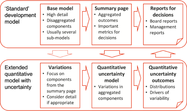
Figure 8 indicates how this might be achieved.

• Property development models usually have a summary page that contains the most important metrics used by managers for operational decisions and the Board for approval decisions. This forms an excellent foundation for quantitative analysis of uncertainty: as well as containing the main decision metrics, it has a familiar and ‘comfortable’ feel for the company.
• The quantitative analysis can then focus on the components in the summary page. Variation estimates for these can be developed readily, considering information from the detailed base model only when it is useful and necessary for forming or justifying a realistic variation estimate.
• Outputs from the quantitative model are based on variations in the components from the summary sheet, so they fit naturally into the ‘standard’ reports used by decision makers. They complement the single-value metrics in the summary sheet with distributions of those metrics (like Figure 4 and Figure 6), as well as indicators of the most important causes of the variability in them (like Figure 5 and Figure 7).

This approach simplifies updating the model when the base case is changed. If it is done well, changes in the underlying data can flow into the risk model with little or even no manual intervention.

In our experience, it is usually necessary to maintain a close relationship between the appearance of a quantitative model of uncertainty and the original property development model on which it is based. Sometimes an entirely new model must be created, but often extending an existing one is necessary for cultural and acceptability reasons, even at the expense of a loss of computational efficiency.

Workshop participation

To ensure that estimates are credible for presentation to the Board, it is important they are generated by people the Board regards as credible and who have appropriate knowledge and insight. To encourage busy senior managers to participate in this case, we set the workshop agenda to allow them to attend when we were analysing the matters for which they perceived they could add most value.

We structured the workshop in three short sessions (Table 4), and we invited executives to attend where they were able. In practice, most participated in all three sessions, an indicator of the strong positive management culture in the company.

In this company, senior executives and the Board placed a high value on understanding risk and how it might affect business outcomes. They expected to have an input to the modelling process, and they wanted to participate actively, so it was important to make it easy for them to attend.

This company had a culture that recognised the importance of sound analysis of uncertainty in all its activities. In other organisations, encouraging senior managers to participate enthusiastically in risk-related activities is an important part of improving culture; making it easy for them to do this is a valuable enabling step.