Introduction

Overview

This paper is set in the context of infrastructure and engineering construction projects. The matters it raises are equally applicable in other fields but to maintain reference to several sectors at once would make the arguments more difficult to follow. The same principles apply to technology systems development and implementation, organisational change, commercial construction and other fields. Only the examples used to illustrate the argument are sector specific.

There is a common practice of referring to general uncertainty in estimates as inherent risk and to major potential disturbances as contingent risk. The distinction is unnecessary and masks important features of project cost uncertainty, as will be explained here. The terms are not used in this paper, except to link the discussion to common practice. All sorts of cost uncertainty are treated as parts of a holistic analysis. The paper examines the structure of cost uncertainty in an estimate and demonstrates how it can be addressed by separating expert judgements from numerical calculations and linking the two together using risk factors that represent uncertainty in major cost drivers. It sets out some principles for deciding what to address by means of expert judgement, what to implement as numerical calculations and how to select the factors that link the two – the inputs to the calculations that are derived from human judgements.

So called contingent risks

Many quantitative risk analyses separate uncertainty into two types referred to as inherent and contingent risks. The term contingent is supposed to signify that a risk might or might not happen so the circumstances it describes have less than a 100% probability of occurring. However, so called contingent risks are often specified with a 100% chance of occurring. In practice these items are just uncertain costs that the analyst cannot, or does not take the trouble to, integrate with the estimate.

Very often, the uncritical adoption of this approach results in poor models that omit important aspects of cost risk. Occasionally, there are potential costs that do sit apart from an estimate and are best modelled in this way, as discrete items, but this is unusual despite the fact that so much project cost risk is described in these terms.

A separate paper will deal with the effect of introducing unnecessary detail into risk models. That is another common practice that not only undermines the analysis process but also imposes an unnecessary workload on the analysts and those whom they need to consult.

Structure

A single risk

If we only want to understand a single well defined risk in isolation, one that really can be separated from other sources of uncertainty, it is not usually very hard to analyse it and build a model to represent the possible outcomes. For instance, if a construction site is known to have serious ground contamination associated with a factory that used to operate there, an assessment can be made of the uncertainty in:

• The extent of the contamination, for example between 20% and 50% of the site with a most likely value of 30% of the site, which is the extent assumed in the estimate, and
• The unit rate for treatment and replacement of contaminated soil, subject to market conditions, say between 95% and 120% of the rate assumed in the base estimate.

There might also be a moderate probability, say 10%, of triggering regulations that will require the site to be treated as if it is all contaminated. The quantity of material in the entire site might be relatively well defined but the uncertainty about the cost of treatment will remain.

This risk can be analysed and modelled, probably resulting in a distribution broadly as shown in Figure 1. The risk is fairly straightforward and would allow a project owner and contractor to understand its financial implications so that they could make provision to cover the cost during project implementation and agree who would be responsible for it.

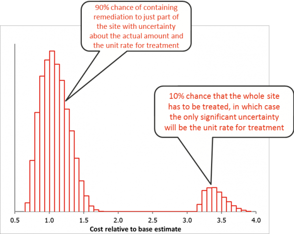
This cost uncertainty is relatively self-contained. As long as it had no material effect on the duration of the project as a whole, it could probably be regarded as a stand-alone element of the cost risk. This cannot be said of the many sources of uncertainty commonly affecting major projects.

Two structural characteristics of the risks in a project are important when trying to assess the cost contingency required:

• Cause-effect relationships, which affect the likelihood or distributions of outcomes arising from uncertainties, and
• Functional relationships, which affect the magnitude of the consequences or impacts of uncertainties as they flow into the cost.

Multiple risks

Root cause analysis is an established method for learning lessons from both successes and failures. The same approach can be used to understand the source of potential future deviations from project plans, that is, the effect of uncertainty on project objectives. Looking for the root cause of risks allows us to focus on what might be done to control the outcome.

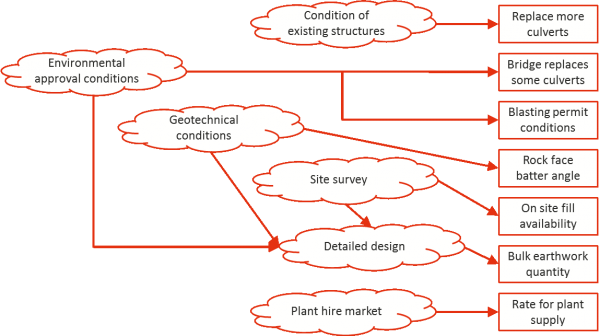
To provide an illustrative example, the following uncertainties could be found in many road or rail infrastructure projects that include waterway crossings and rock cuttings:

• More existing culverts than expected could be in poor condition and have to be replaced
• One group of culverts in the baseline design may have to be replaced by a bridge to achieve the required hydrological performance
• The rock face in a cutting might have to be at a shallower angle than assumed to achieve stability requirement
• Blasting permit conditions could force the project to use smaller charges for noise control, reducing productivity in the cutting
• The project may be unable to find all the fill required within the permit area so fill has to be bought in
• Detailed design work could lead to variation in bulk earthworks quantity
• Supply of earthmoving machinery may be affected by work on other projects in the immediate area so it has to be sourced from further away at higher cost

Details will vary from one project to another but the reasons for uncertainty about these matters could be as illustrated in Figure 2. The cloud symbols represent information that is not fully defined at the time the estimate is prepared.

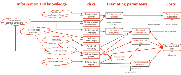
It is common to analyse such risks separately from one another, as with the example described in Section 2.1. This is often unrealistic and undermines the integrity of the process very badly. To see why, look at the next stage of cause-effect relationships describing the consequences of the risks on the project cost, which is illustrated in Figure 3. As before, details will vary from one project to another.

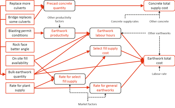
The costs and cost drivers shown here will be affected by other factors not included in this simplified picture. Some of these are indicated by the notes linked to the costs and parameters using dotted lines.

The effects of the risks overlap with one another. For instance, the risk relating to culverts and the rock cutting could have implications for the general bulk earthworks quantity uncertainty and several of the costs and parameters, the items shown in black round cornered boxes with red text, are affected by two or more of the risks that were initially identified. At the very least, some attention to the boundaries between the risks and a mechanism to represent the interactions is required if the risks are to be modelled as individual items.

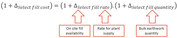
Not only is it necessary to think about several parts of the cost when assessing the immediate consequences of these individual risks but these consequences themselves interact. For instance, the extent to which the cost is affected by a variation in labour productivity, subject to blasting permit conditions and possibly other matters, will depend on the amount of work to be done, dictated by the bulk earthworks quantity and availability of on-site fill. To understand the effect of one risk it is necessary to understand the consequences of the others affecting the same part of the cost, as illustrated in Figure 4 where Δ represents the fractional variation in a value relative to the base estimate.

Combining Figure 2 and Figure 3, in Figure 5, highlights the degree of complication at work in the cost uncertainty.

These risks were not deliberately selected to ensure a high level of complication in the illustration. They are a small selection of risks that could arise in a road or rail infrastructure project with waterway crossings and a rock cutting. The apparent simplicity of the original list of seven individual risks does not reflect the real nature of the uncertainty in the cost estimate, it is a lot more complicated than seven independent risks that can be analysed in isolation from one another. These examples are only a small part of what might arise in an entire project yet some characteristics are clear:

• The risks affect one another
• The risks share common root causes in the information and knowledge available to the project
• The consequences of the risks are multifaceted, some affecting several estimating parameters
• The consequences of one risk may be affected by the consequences of other risks that affect the same estimating parameters, that is they interact, as with quantity and rate uncertainty for a bulk material.

This structural complexity cannot be ignored if the analysis is to be realistic.

Default approach

Risk event modelling is the backbone of what has become the default approach to project cost risk assessment for contingency analysis. The events are almost always treated as independent uncertainties with no attention to any interactions between them or to a shared dependence on common sources of uncertainty.

It is worth asking why so many project cost risk assessments tackle a complicated system such as that illustrated in Figure 5 without taking account of the interactions between risks and the effect of common sources of uncertainty. By leaving out the interactions and dependencies between sources of uncertainty, the default approach creates unrealistic models.

One reason the default approach persists is no doubt the fact that the practice of listing risks and evaluating them each separately has been in use for a long time. It has become so familiar that it no longer attracts critical thought. Engineers and others who started working this way before computers were generally available were confined to methods that could be carried out with pen and paper using log tables, slide rules or, later, four function (+ - x /) calculators. They had little choice.

The sense that analysing separate risks independently of one another is the right way to assess contingency requirements has become accepted to the point where no one stops to think whether it is the best option now that we have powerful computers at our disposal. This acceptance of common practice is passed on to new generations of engineers and analysts in formal education and in workplaces.

The basic structure of traditional models is the same as it would have been in the nineteen sixties. They now reside in a computer instead of on paper. Professional guidance, by experts and professional societies entrained in past practices, rarely if ever suggests that the cause-effect structure and interactions of risks should be taken into account when designing a model.

The simplistic risk event structure for cost uncertainty modelling is used because it has always been used. Monte Carlo simulation is very powerful, flexible and easy to apply with the inexpensive simulation tools that are available now. Using it to animate what could almost be a paper based model, with events that can occur or not in place of expected value calculations (Expected Value = Probability x Impact), and to replace fixed impacts with distributions of outcomes, is an almost trivial application of the method. It may look sophisticated but is often over simplified.

From estimate to contingency

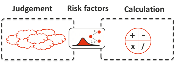
Judgement and calculation

Human judgement plays a large part in any contingency assessment as it does in estimates. No matter what approach is used to understand project cost risk, judgement is required to assess the probabilities of events and the ranges of distributions. The overall analysis consists of judgements linked to numerical calculations as illustrated schematically in Figure 6.

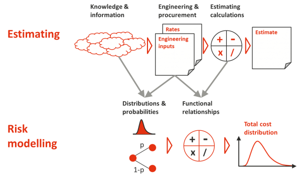
The design of a model effectively allocates some matters to be addressed by judgement and some by numerical calculation. For instance:

• Judgement is required to assess event probabilities and the potential variation in estimate parameters, and
• Numerical calculations can be used to calculate the variation in labour hours from the variations in material quantities and in labour productivity.

So called contingent risk modelling relies on judgement to assess the probability of a risk occurring and the range of values its impact could take on but generally does not address the interrelationships and dependencies that have been discussed earlier. In addition to important relationships being left out of the analysis, this has two consequences:

• Knowing that there are interactions and dependencies at work, even if they are not explicitly spelled out, people will try to make up for these missing aspects of the analysis by adjusting the parameters of the risk event structure, the consequence distributions and probabilities
• Being faced with a complex cognitive task, trying to make sense of a complicated system in terms of a simplistic model, people are unable to make a reliable connection between the real nature of the uncertainty they face and the way it is represented in the analysis so their judgement on this matter cannot be relied upon to the same extent as their judgement about their core areas of expertise such as engineering or estimating.

Calibration and adjustment

It is common for people to look at the first outputs a model produces, for a single risk or a whole project, and find that it is not what they expected. The analysis might suggest a contingency they regard as either too small or too large. They will then try to reconcile the model output with their expectations.

Models are a means to investigate a system, not a source of absolute forecasts. It is quite reasonable to question conclusions that differ from expectations and either:

• Where a model is found to be incorrect, adjust the model, or
• Where the model is persuasive, use it to calibrate judgements.

This balancing process is an important part of modelling but it falls apart if the model is weak or incomprehensible. If the model is so fluid that no one can say whether it is realistic or not, except by examining the outputs, only the model adjustment side of the balancing process will be in effect. A weak model will be unable to stand up to experienced judgement and gut feel will be given more weight than the analysis, rendering the analysis futile.

A similar problem arises when a model requires people to make assessments that they find very difficult. If the relationship between the real project and the model they are asked to use is unclear, people will look for points of reference outside the project itself to guide them. They will look for something to help them work out what the answer should be. More often than not, they will gravitate towards an outcome they or their peers expect to see whether it is realistic or not. Once again, they will adjust the model to fit the outcome they expect.

The gulf between the complicated nature of most projects’ cost uncertainty and the simplistic nature of risk event models means these models are susceptible to being adjusted to fit expectations. At its worst, the exercise will become window dressing to justify a result that has been arrived at by other means or to support a preferred outcome that was established in decision makers’ minds before the analysis began.

Robust modelling

A robust model that will expose unrealistic expectations and will challenge biased or conflicted assessment must:

• Limit the complexity of the human judgements it requires, so that these judgements can be made reliably, and
• Use numerical calculations that are closely aligned to the real world behaviour that they represent.

A robust model design will ask those producing the inputs to describe uncertainty in terms that make sense to them. This means that a predefined structure cannot be imposed. It has to fit the project and the way people understand it.

The structure must be developed with regard to the way the people who understand the project think about the cost and the uncertainty affecting it. Having said this, there is a fair degree of common practice in the way estimates are developed for road and rail infrastructure projects. This means that common model structures can at least provide a useful starting point for a new project.

If the structure in Figure 5 is redrawn without the simplistic risk events, making connections directly from the uncertain areas of knowledge and information to the estimating parameters, it might look as shown in Figure 7.

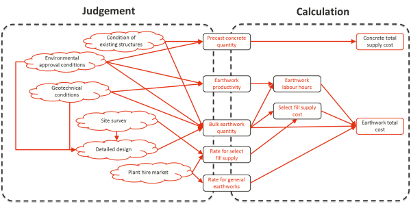
To the left is the web of knowledge and information that a project team understands about their work. There is a point at which it is more useful to ask someone with suitable experience to make an assessment than it is to try to decompose and model the factors at work. For instance, trying to analyse the relationship between an existing site survey, its strengths and weaknesses, and the state of the design in a way that will help quantify the cost risk is unlikely to be rewarding. The analysis would soon become very bulky, with a large number of interconnected factors, and it would absorb more effort than the extra value it might deliver.

In contrast to the left hand side, the estimating parameters and relationships shown on the right are relatively clear and easy to model. Variations in the quantity of earthworks and in labour productivity can be used to calculate a variation in the labour hours required to carry out the earthworks and this is quite straightforward. Similarly, variations in the quantity and rate for select fill can be used to calculate variation in the cost of select fill and this can be added to other earthworks cost variations.

The design of a model for a specific project might not use the same relationships as shown here. It will depend on the details of that project and how the team implementing it has decided to develop their estimate and carry out their preliminary studies. This means that two very similar projects implemented by different teams might be addressed differently.

The design of a model can be summarised in the form illustrated in Figure 8.

Calculations, on the right, typically take much the same form as they do in routine estimating. Quantities, unit rates, overhead running rates, durations, and lump sum costs are combined using basic arithmetic operations. This usually takes place within a Monte Carlo simulation process that aggregates the various uncertain values and events represented by the risk factors.

Knowledge and information, on the left, is incorporated into the analysis by drawing on the judgement of the project team and subject matter experts who assess probabilities and distributions that define the risk factors used as inputs to the calculation. Their assessments are integral to the process and must be derived with a view to avoiding bias and ensuring that they leave nothing out.

The risk factors that link the two parts of the process must be chosen to be as straightforward as possible so that they can be assessed reliably. It is relatively straightforward to assess uncertainty in the unit rate for a bulk material, the quantity of a single type of material, the labour rate, labour productivity and similar factors. There are generally no complex interactions to be considered in making this sort of assessment. By contrast, assessing the uncertainty in a material cost subject to uncertainty in both the quantity of material and the unit rate for the material is more difficult. Taking account of two uncertainties and an interaction between them, as illustrated in Figure 4, is a significant challenge that few if any people can meet. If a cost is made up of several distinct materials that are all subject to different levels of rate and quantity uncertainty, the process becomes even greater and even less likely to result in a reliable assessment.

For physical infrastructure projects, experience has shown that a useful set of risk factors to consider as a starting point are the uncertainty in:

• Bulk material quantities
• Bulk material unit rates
• Labour productivity
• Labour cost rate
• Construction plant productivity
• Construction plant rates
• Overhead running rates
• Duration.

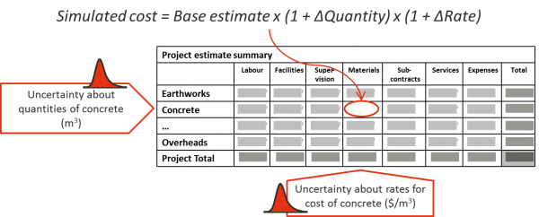
An illustration of the way this has been used for some projects is shown in Figure 9. Only one cell’s calculation is shown but similar relationships would be implemented in other cells. Very often, the influence of a bulk material quantity’s variation will be applied to most items across a row, especially labour, bulk materials and supervision or contractors’ overheads. Productivity and labour rate uncertainty will be applied to the labour costs column as a whole unless different classes of labour are subject to different levels of uncertainty. The uncertainty about unit rates for each of the disciplines will often be different from one discipline to another although they might be correlated by a common dependence on market conditions.

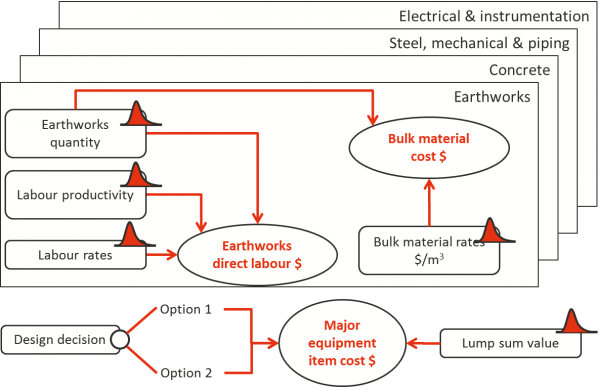
A model based on these principles might have a structure similar to that illustrated in Figure 10. The risk factors are those with a distribution curve icon. The remainder are calculated values. This example also includes a discrete risk, a design decision, which truly does sit aside from other risks.

Conclusion

The structural relationships between sources of uncertainty, estimating parameters and costs can be complicated. Simplistic risk modelling structures often fail to allow for the interactions and dependencies that link them together. A conscious decision can be made about which parts of the analysis to address as judgements and which to model with numerical calculations. Attention to this decision can:

• Simplify the assessments required, avoiding unnecessary complexity that will make it difficult to obtain realistic inputs to a model
• Integrate into the model the interactions between sources of uncertainty
• Reduce the chance of a model being over ridden for invalid reasons when it challenges pre-existing expectations.

The three components of a sound structure for a cost risk model, reiterated in Figure 11, are:

• The matters that will be addressed using the judgement of the project team and subject matter experts
• Risk factors that are assessed by reference to the knowledge and information held by the project team and subject matter experts that are then used as inputs to the calculations
• Straightforward numerical calculations that link the inputs to subtotal and total costs and the variation in those costs.

This structure is not the same for all projects and is not predefined for any project. It represents a set of design decisions that an analyst can make to fit a model to a project, to its estimate and to the people who have the knowledge to provide the inputs to the model.