Simple schedule risk modelling with Safran Risk
Introduction
With a view to exploring alternative tools for quantitative project risk assessment on major engineering projects, Broadleaf reviewed Safran Risk, a tool for project planning and for modelling schedule and cost uncertainty. While Broadleaf does not endorse any specific tools, we use several in our work and discussing their application provides an opportunity to offer insights into not only the features of those tools but quantitative risk assessment and modelling in general.
This is the first in a series of notes. This one deals with simple schedule risk modelling. Later notes will address integrated schedule and cost risk modelling with a simple schedule, more complicated schedule networks, the use of probabilistic calendars to model work interruptions and special modelling constructs that can be useful with some projects.
We have approached this review in the context of major civil engineering, mining and resources projects that form a large part of Broadleaf’s activity.
Example project
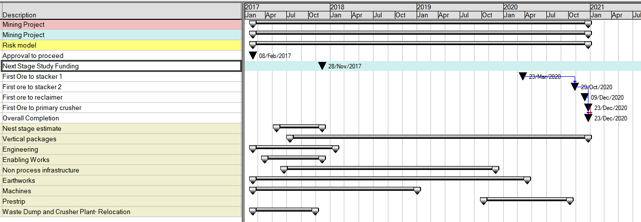
The review was conducted using a plan of a mining project that had been developed for that project’s study phase. It had been subjected to a schedule risk analysis using a widely known schedule simulation package to evaluate the model. Being part of a feasibility study, the plan was relatively high level. The model network features are summarised in Table 1. A rolled-up view of the model is illustrated in Figure 1.
|
Activities |
56 |
|
Uncertainty factors |
11 |
|
Overall duration |
47 months |
For this review, the model created for the original analysis was replicated in Safran Risk.
Figure 1: Gantt summary
Background
Purpose
Broadleaf uses project schedules as source material for schedule risk models, which are often linked to a cost risk model. Broadleaf specialises in risk assessment and this review focuses on that aspect of the Safran Risk package.
Approach
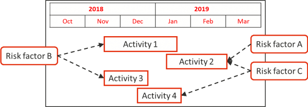
Our schedule risk assessments generally use a model network that is consistent with the master schedule while being somewhat smaller and, in most respects, less detailed than a full project schedule. We examine the factors driving schedule performance, map these onto the activities they affect (Figure 2), assess the range of values each factor could take and represent that range with a distribution of values in the model. In general, one risk factor will apply to more than one activity and one activity may be affected by more than one risk factor. The risk factor formulation avoids the need to wrestle with complicated correlations that arise in other forms of modelling such as line item ranging and risk event modelling, as discussed in a longer paper by Broadleaf. The models are evaluated by Monte Carlo simulation
Figure 2: Activities and risk factors
We occasionally facilitate the development of an initial high-level network to enable an early schedule risk assessment where the client has not yet prepared a formal schedule. Whichever modelling tool we use must be compatible with commonly used scheduling software, easy to use and capable of clearly displaying the model for others to understand, interrogate and accept.
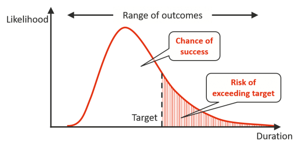
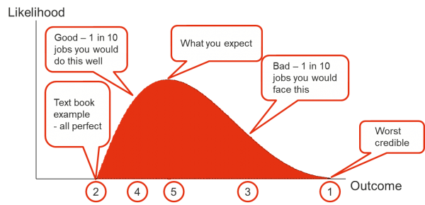
Our approach to estimating the range associated with an uncertain quantity or factor, illustrated in Table 2 and Figure 3, has been developed in consultation with major clients to limit bias in the assessment. It is based on exploring the context and background of the uncertainty in a quantity first, then describing pessimistic and optimistic scenarios and only then making a numerical assessment of the range of the uncertainty. The numerical assessment starts with the extreme worst and best forecasts. These values are often unreliable because they represent very low likelihood outcomes, but thinking about them opens up the assessment and helps to avoid anchoring bias. We then assess pessimistic and optimistic values, having a nominal ten percent chance of being exceeded or bettered respectively, P90 and P10 values, and finally the most likely value. The P10, most likely and P90 values are used to define a distribution in the model.
Table 2: Workshop data capture
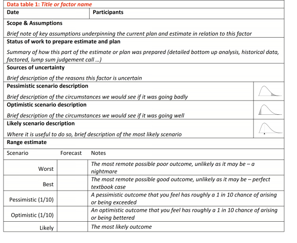
Figure 3: Elicitation sequence
Simple schedule model
An XER file from the original model was exported and read into Safran Risk. Ten risk factors, representing possible variations in the duration of particular types of work, and one uncertain duration expressed directly in days were used to represent the uncertainty in the schedule. These did not form part of the XER file. They were added manually.
Some tools separate discrete risks, those with a probability of occurrence less than 100% that might also have an uncertain level of impact, from sources of uncertainty that will definitely affect a project where only the magnitude of their impact is uncertain. Both can be implemented in Safran Risk using the Project Risk window.
The risk factors used in the model are shown in Table 3, where the numbers in brackets are the minimum, most likely and maximum values used in the original model.
|
Factor |
Parameters |
|---|---|
|
Procurement progress - general |
(97, 100, 127)% |
|
Procurement progress - earthworks |
(81, 100, 130)% |
|
Procurement progress - power conditioning |
(64, 100, 122)% |
|
Procurement resourcing risk |
(30, 49, 62) days |
|
SMP E&I progress |
(81, 100, 141)% |
|
Engineering progress |
(78, 100, 156)% |
|
Earthworks progress |
(81, 100, 141)% |
|
Stacker reclaimer delivery progress |
(80, 100, 170)% |
|
Major machinery delivery progress |
(80, 100, 133)% |
|
Contractor and external delays |
(98, 100, 119)% |
|
Owner team productivity |
(96, 100, 137)% |
Many abbreviations common in the mining sector have been removed from the original schedule to make the material accessible to those who are not familiar with the terms. However, two abbreviations have been retained to avoid unduly long labels in the figures:
- SMP – structural mechanical and piping
- E&I – electrical and instrumentation.
Some of the activities and one of the risk factors relate to the construction work associated with SMP and E&I. In this case, a single risk factor was used to describe uncertainty in the rate of progress in SMP and E&I tasks.
All the distributions were modelled in Safran Risk using triangular distributions as they had been in the original model. This is illustrated in the screenshot in Figure 4 showing details of just one of the risk factors. Since the software used for the original model requires inputs in the form of a minimum, most likely and maximum value, the P10, most likely and P90 values had been converted to equivalent minimum, most likely and maximum values that define the same triangular distribution as the P10, most likely and P90 values.
Figure 4: Risk factor specification
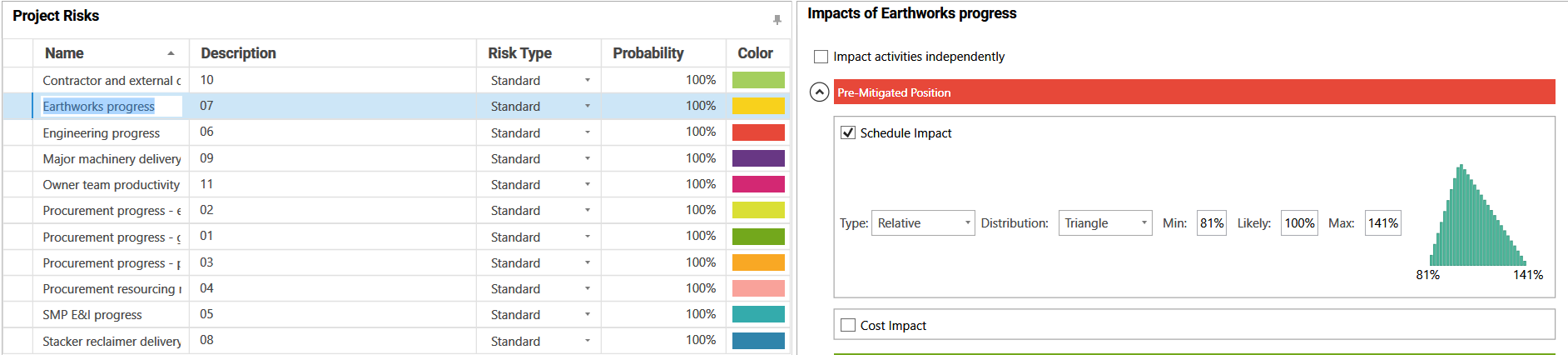
We prefer to define distributions using the P10 and P90 values assessed using the process described earlier as this preserves a transparent relationship between information provided by those making the assessments and the model. Safran Risk allows for uncertainties, whether described as percentage variations or directly in days duration, to be defined using percentiles as well as with minimum and maximum values. Safran Risk supports other forms of risk modelling including modelling calendar-based uncertainties.
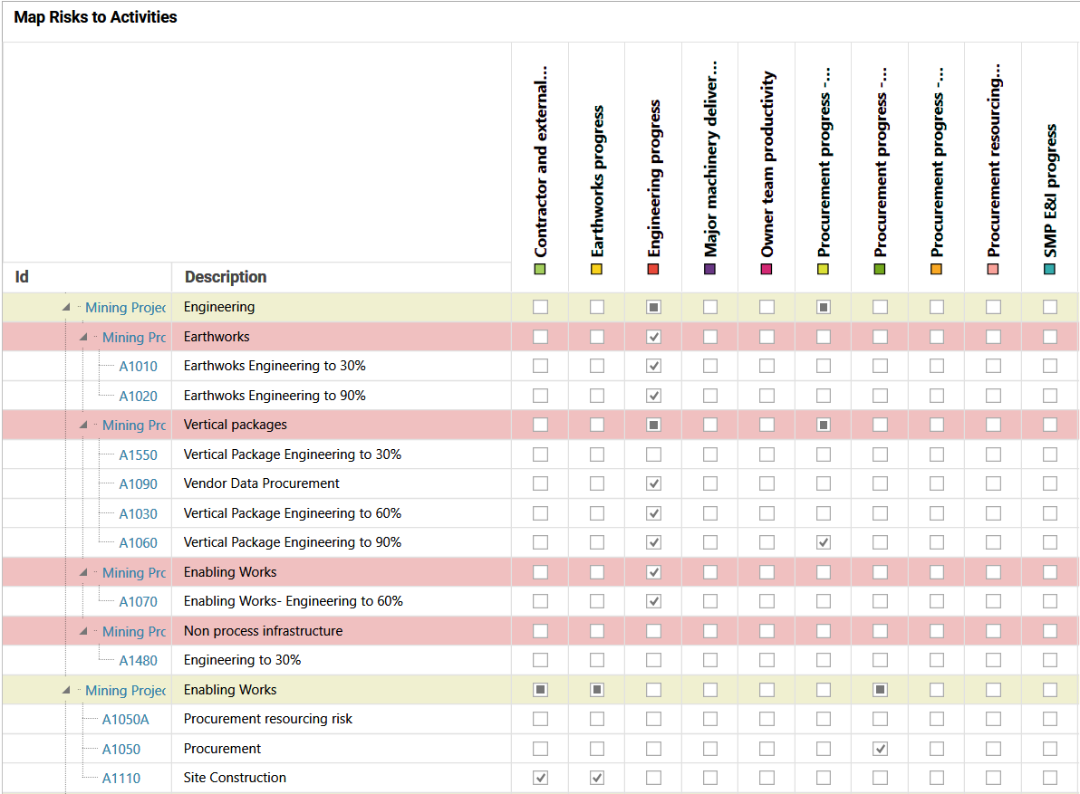
The risk factors were allocated to activities in the model. Safran Risk has a risk mapping facility, illustrated for a few activities in the screenshot in Figure 5. Factors are allocated to activities simply by ticking a box in the activity’s row and the risk factor’s column.
Figure 5: Risk mapping
With the model network in place, the risk factors defined and allocated to activities, the model was complete.
Outcomes
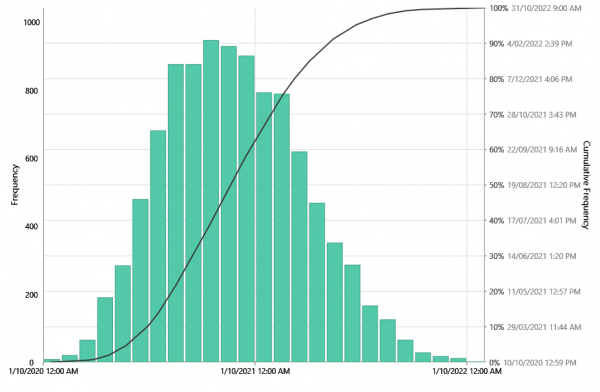
The model was evaluated through ten thousand iterations. This took a few seconds in Safran Risk compared to a few minutes in the software used for the original analysis. The results in Safran Risk, see the screenshot in Figure 6, were compared with the original model at the P10, mean, P50 and P90 points on the overall project duration distribution. They matched very closely, within five days or less.
Figure 6: Output distribution – total duration
Safran Risk offers useful analysis capabilities for investigating the outcome of a model and the relationships between the inputs and output distributions.
Correlation sensitivity takes the values used as inputs, the samples generated for each of the risk factors during, in this case, ten thousand iterations, and the output for each of those iterations and calculates the correlation between each input and the output. If the output always increases when a particular input takes on a high value, and vice versa, we know that this input has a strong influence on variations in the output. If the output is as likely to rise as it is to fall when a particular input rises, that input is clearly not very influential. This mechanism is provided in many Monte Carlo simulation tools including @RISK, a popular tool for modelling cost risk.
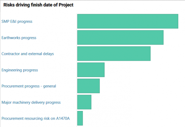
For the model described here, the correlations between variations in each of the seven most influential inputs and the variation in the overall duration are shown in the screen shot in Figure 7. The top three items appear to dominate the uncertainty in the end date, the spread of results in the model output. This can be a valuable guide to directing study effort to narrow the forecast of a project’s outcome by improving the accuracy of estimates used to prepare the schedule. That might be achieved by obtaining better information, by increasing the degree of control the project can exercise, or by reducing the project’s sensitivity to a particular uncertainty, perhaps by taking the activities it affects off or further off the critical path.
Figure 7: Uncertainty sensitivity
There is no guarantee that making the outcome more predictable will make a project more attractive but increasing the certainty with which the outcome can be forecast often simplifies decision-making.
The machine on which this trial was run only has 4GB of RAM and it was necessary to limit the number of iterations of the model to be able to use Safran Risk’s second form of sensitivity analysis, which assesses the impact of each risk factor separately, see the screenshot in Figure 8. This form of analysis shows how much the end date of the project will change if each risk factor is removed and all the others are left in place. In this case, the differences in end date were calculated at the mean of the associated distributions.
Figure 8: Impact sensitivity
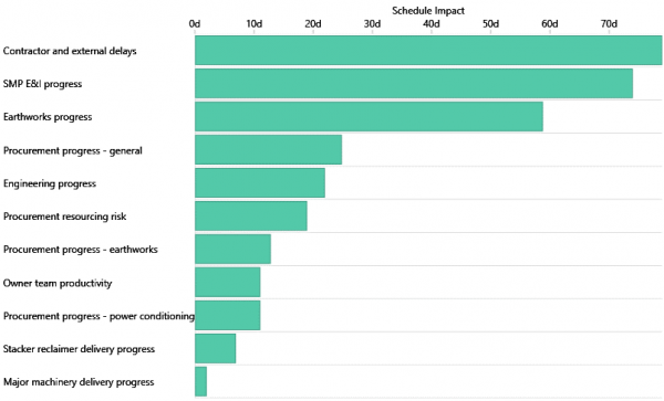
While the uncertainty sensitivity in the screenshot in Figure 7 shows where to devote effort to reduce uncertainty in the outcome, the impact sensitivity in Figure 8 shows how much scope there might be to improve the mean end date if each of the uncertainties were to be controlled more closely. There are clearly three areas where schedule improvements might be targeted by seeking to control the uncertainty affecting major parts of the project. It is not a recipe that can guarantee a shorter schedule but it is a good guide as to where to focus attention if a shorter schedule is important.
Conclusions
The exercise described here sought to replicate in Safran Risk the development of a model previously prepared in another widely used package, starting with an XER file of the activity network and definitions of risk factors. It proved very easy to do aside from the normal challenges of learning to use a new software package. Some of the features that came to our attention during this exercise are set out in Table 4. The package offers many features that have not been used in this exercise. In particular, cost risk was not modelled here.
|
Features |
Comments |
|---|---|
|
Importing an existing network |
The XER file from the original model imported as expected. Safran applies default formatting to the labels and Gantt chart bars but the formatting can be modified. As often happens when moving between schedule tools, some milestones were moved by a day, from the end of one day to the start of the next day. |
|
Defining risk factors |
The project risks window is easy to use and provides a graph of the distribution being defined as well as space to make notes. This could be used in a workshop setting to engage participants in the specification of risk factors. Broadleaf would always recommend the structured approach described earlier, establishing the context, exploring pessimistic and optimistic scenarios and assessing quantitative measures of uncertainty using a method that will help avoid anchoring bias. In addition, making notes of the rationale for an assessment after specifying a range in quantitative terms lays the process open to confirmation bias, fitting the description to the numbers that have been entered rather than exploring the roots of the uncertainty and then quantifying it. Safran Risk offers several distribution shapes. Among these are two forms of the common triangular distribution, one based on minima and maxima and the other based on high and low percentile points. There is a facility to define a distribution in terms of cumulative distribution points as well as a selection of standard distribution functions. The risk factor definitions, labels and numbers can be exported and imported to and from Excel. In a larger model, this may be useful to make global edits and to enable stakeholders to scan a table quickly to examine the ranges that have been used in a model. It would be useful to be able to do this from within Safran Risk but the Excel interface provides an alternative. |
|
Linking risks to activities |
The risk mapping window provides a matrix with activities on one axis and risks on the other. This is a natural format for making the connections between risks and activities, which mirrors the way we often present this information in reports. It would be useful to be able to export the matrix in a form that could be included in a report or sent for review to stakeholders who do not have Safran Risk, perhaps as an Excel sheet. |
|
Evaluation of the model |
The Monte Carlo simulation evaluation runs very quickly. Safran Risk proved to be fairly resource hungry although it ran well on a Windows 10 PC with an i7 2.8GHz processor and 4GB of RAM. |
|
Simulation outputs |
Results are presented in a tabular summary of key values and as a histogram and cumulative distribution of end dates. The graph can be copied for pasting into a report and the raw data can be exported into an Excel file for bespoke processing if this is desired. |
|
Sensitivity analysis |
The risk driver or correlation based sensitivity analysis is a common feature of Monte Carlo simulation tools. The tornado chart can be copied for insertion in reports. The impact analysis option Safran Risk offers is not common and is a very useful feature. It automates what is otherwise a laborious manual task of excluding sources of uncertainty one by one, evaluating the model with all the other risks still in play and comparing the result to the model with all of them in play. |
|
Navigation and workflow |
The layout of the modelling and analysis windows is very helpful with a natural flow from left to right. |
As with any tool, good results depend on being able to design a realistic model and obtain meaningful assessments of uncertain factors from those who know a project. No tool will make up for a poorly formulated model but a sound model can be implemented in most modelling tools, some more easily than others. Leaving aside the challenge of getting to know a new package, Safran Risk proved easy to use as a risk modelling tool.
Later reviews will address other features of modelling project risk using Safran Risk including cost risk modelling.
On our web site there are many papers about risk modelling methods as well as case studies describing practical applications. To keep up to date with our work, please subscribe to our monthly newsletter.