Construction costs for a portfolio of buildings
Summary
A national construction company was part of a consortium bidding for a public private partnership (PPP). The winning bidder would have to deliver a large number of dwelling units at sites across Australia, and maintain them for an extended period. We worked with the contractor to develop a quantitative model of the uncertainty in the design and construction (D&C) costs for the project.
The D&C model was based on a standard design and a Bill of Quantities (BoQ) that had been developed centrally. It took into account common features and common sources of uncertainty across all sites, as well as regional variations. We conducted workshops with the regional estimating teams to analyse variations in quantities and rates.
Operating and maintenance was analysed separately and is not described in this case study.
Base estimate and model
The company’s central project team had developed a standard design and a standard Bill of Quantities (BoQ). These were used as a base for the quantitative model, augmented with information about sources of uncertainty. The quantitative model referred to the BoQ for each site, with results aggregated at regional level, and aggregated again at national level.
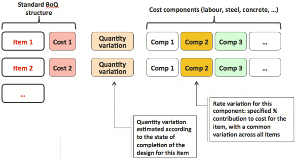
For any specific site, Figure 1 outlines the model structure:
- The costs of items in the BoQ were estimated through the company’s standard process
- Quantity variations were estimated according to the degree of completion of the design for the item
- Each item was disaggregated into a set of cost components, each specified as a percentage of the total cost for the item, and a rate variation was applied to each component throughout the estimate.
Figure 1: Model structure overview for a site
Direct costs: quantity variations
Quantity variations were related to the expected completeness of the design at the time of the initial estimate, taking into account site-specific characteristics that impinged on the design (e.g. geotechnical characteristics). These were assessed for individual items in the BoQ.
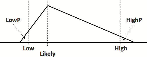
There were five quantity variation categories, each expressed in terms of a proportional change from the base estimate and described in Table 1. Each category was interpreted in the form of a triangular distribution with confidence bounds (Figure 2), with low, likely and high values shown in the table. Quantities for Category A were certain, but there was a wide spread for Category E items where the design was less complete or there were greater unresolved uncertainties. Selected distributions were used as multipliers for the associated item costs.
In general, in the initial model:
- Items above foundation level were expected to be in categories B or C
- Below-foundation items were expected to be in categories D or C.
|
Category |
Interpretation |
Low |
Likely |
High |
|---|---|---|---|---|
|
A |
Complete, not subject to any quantity variation (e.g. for specific identified items) |
1 |
1 |
1 |
|
B |
Excellent, very close to final design |
0.95 |
1 |
1.05 |
|
C |
Good, sound design basis for estimating |
0.95 |
1 |
1.15 |
|
D |
Moderate, fair design basis |
0.90 |
1 |
1.30 |
|
E |
Poor, many uncertainties |
0.90 |
1 |
1.50 |
The initial model reflected the initial workshops, when the design was at an early stage. As the level of detail of the design improved, the original values were judged to be too conservative and the quantity variations were adjusted from the original values. In many cases design categories C and D were improved by one category and E was improved by two categories as the design progressed. By the time the estimate was finalised, there were no items where the category was lower than C.
In the model, the values of LowP and HighP in the triangular distribution in Figure 2 were set to 10% and 90%, so the range between Low and High was interpreted as a 80-percent confidence band. (We used the Trigen function in @Risk.)
Figure 2: Triangular distribution
Direct costs: rate variations
Rate variations were related to the unit prices of the main components of each item in the estimate: labour, steel, concrete and so on. By identifying the main components, the effects on the estimate of common drivers like labour rates or the price of concrete could be assessed.
The labour and non-labour components of standard items in the BoQ were obtained from estimating sheets for sub-contractor negotiations. It was assumed that the components would be the same for each item in the BoQ, irrespective of location.
The variation associated with each driver was assessed in terms of low, likely and high values. As for quantity variations, the low and high estimates were interpreted as 10- and 90-percentile values.
The components with associated rate drivers were:
- Direct labour rate and productivity variation
- Steel materials supply price variation
- Concrete materials supply price variation
- Formwork materials price variation
- Earthworks price variation, including equipment but excluding labour
- Fit out materials supply price variation, including items purchased in more-or-less finished form
- Plumbing materials price variation
- Mechanical items price variation
- Electrical materials price variation.
The working assumption was that rate variations for a component would be consistent through the estimate for any site. For example, it was assumed that a proportional labour variation could be assessed that would be applicable for all labour skill groups, irrespective of the base hourly rates that applied to each group.
Direct costs: total variation
The variation for each direct cost item was calculated as:
- Base estimate value, multiplied by …
- Quantity variation, according to the state of the estimate and the design for the item, multiplied by …
- Rate variation, calculated as the sum of the proportion of the price attributable to each component multiplied by the associated component rate variation.
Preliminaries and indirect costs
Quantity and rate variations for preliminaries were estimated using the same process as for direct costs. The rate variation drivers for Preliminaries were:
- Preliminaries supervision rate variation
- Preliminaries labour rate variation
- Preliminaries plant hire or lease rate variation
- Preliminaries sub-contract and materials rate variation.
Indirect costs were included at the values provided by the estimating team.
Fixed and variable costs were also identified, to facilitate testing of the sensitivity of the estimate to variations in the construction delivery from the planned schedule. Escalation was treated separately, outside this model.
Correlation between rate variation drivers
When distributions are combined, it is important that correlation is estimated appropriately; if not, the outcome distributions tend to be too narrow and a substantial portion of the variation may be omitted. For this estimate, common drivers of variation were isolated and assessed explicitly, and their effects on other parts of the estimate were included arithmetically.
It was likely that the drivers for rate variations would be correlated, as they were all driven by common factors, including national and regional economic conditions and levels of demand for resources. It was expected that the costs of most items would rise or fall together according to the ‘heat’ of the market, a common phenomenon in many projects.
The estimating uncertainty model used explicit correlation coefficients for rate variations. Most correlation coefficients were set to 0.7, which provided a modest level of dependence. The exception was the coefficient that linked labour rate variations to supervision rate variations, where a higher correlation of 0.9 was assumed.
These coefficients were set as parameters in the model, so the effect of different correlation assumptions on the results could be tested.
Indirect costs
Indirect costs were included at the values provided by the estimating team. For the variation model, the contingency component of the escalation was omitted.
Specific discrete risks
A range of specific risks was considered, from an extensive risk register. Most of them were included in the analysis as contributors to the quantity and rate variations. Some led to changes in the design as the work progressed and contributed to reductions in variability. A few were set aside for special treatment by the commercial negotiating team as matters to be addressed in the contract.
Workshop process
Elements of the estimate, model and risk structure were developed and reviewed in a series of workshops around Australia. The initial workshops were very detailed, as we built up an understanding of the design, the work required for construction, the general sources of variability and any discrete risks that needed to be addressed through adjustments to the design or to the planned approach to construction. Later workshops focussed on local and regional variations.
Table 2 shows an edited version of a data collection template. The aim of the workshops was to stimulate expansive thinking about what might happen, and to document the discussion in a reasonable level of detail that would facilitate easier updating as design and planning work progressed and the project moved towards PPP contract closure.
Table 2: Direct labour rate and productivity variation
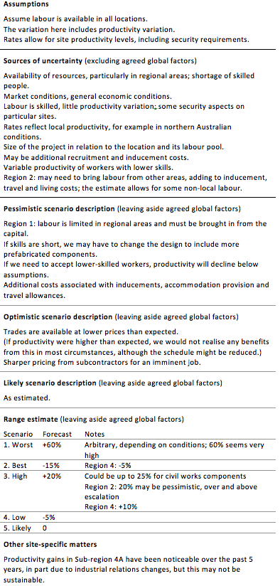
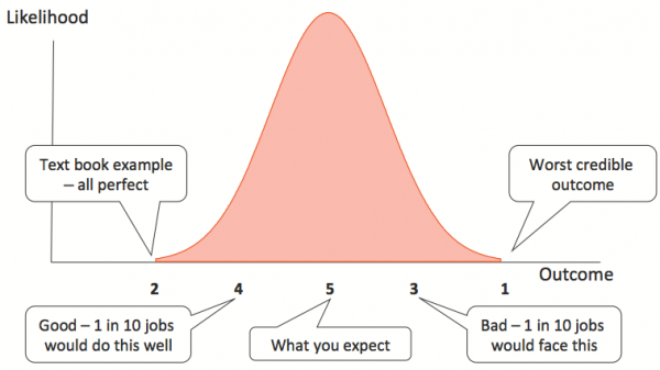
The range estimate in Table 2 merits further discussion. The sequence in which values are estimated, shown in Figure 3, is important. It is designed to reduce some of the more common biases when data are estimated.
- We started by encouraging workshop participants to imagine the worst credible outcome and the best or ‘perfect’ outcome, labelled 1 and 2. The purpose was to expand the group perspective on what might happen, and hence counter the common over-confidence bias – we all think we are better at estimating and doing the work than we really are, and this often leads to estimated ranges that are far too narrow.
- We then asked for the pessimistic and optimistic outcomes, labelled 3 and 4, and a description of scenarios in which they might come about. We defined the pessimistic and optimistic scenarios as those that might arise in about one in ten jobs – we wanted the scenarios to be understandable and within the experience range of seasoned estimators and project personnel, so they could have more confidence that the estimates were grounded in what might really happen. (The very worst and the best cases discussed above can be imagined, but few if any people will have experienced them.)
- Finally we asked for the most likely value, labelled 5. Discussing and estimating this value at the end, combined with the scenario descriptions, was designed to avoid the anchoring and adjustment bias. This bias arises when values are estimated in sequence – the first value becomes the anchor, subsequent values are formed as adjustments from the first one, and in most cases the adjustments are too small. This leads to range estimates that are far too narrow and generates a consistent under-estimation of potential variability.
Figure 3: Developing a range estimate
Correlations between variations were also discussed in the workshop. The general assumptions about correlations noted above were examined for ‘reasonableness’ and their application in each regional market.
Outcomes
The original results were based on the original design status, which included significant variation, but the design was a work-in-progress and its level of detail increased substantially during the course of this analysis. As the design improved, the quantity variations in the model were adjusted to tighter ranges. This reduced the contingency, calculated as the difference between the P20 value and the base estimate, from about 12% to about 7%.
Figure 4 shows the distribution of direct costs aggregated across all sites, after including design improvements. The outcomes are summarised in Table 3. (The values have been normalised to preserve confidentiality.) If an overall confidence level of 80% of achieving a target budget were required, shown as a P20 probability level in Table 3, then the direct cost contingency should be about 7% of the base cost estimate value excluding the original contingency. There was a 76% chance of exceeding the base estimate value excluding the contingency. There was a 48% chance of exceeding the base estimate value including the contingency in the original estimate.
|
Measure |
Normalised value ($) |
Variation ($) |
Variation % |
|---|---|---|---|
|
P90 |
978 |
-22 |
-2% |
|
Base less contingency |
1,000 |
- |
0% |
|
P50 |
1,031 |
31 |
3% |
|
Mean |
1,034 |
34 |
3% |
|
Target P20 |
1,071 |
71 |
7% |
|
P10 |
1,091 |
91 |
9% |
Figure 4: Direct cost distribution, all sites
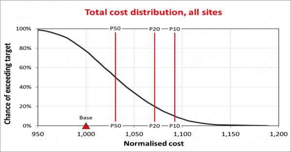
The principal drivers of variability in the direct cost were variations in the rates for supervision and direct labour, which included variability associated with labour productivity, and quantity variations associated with design uncertainty and variability.
(Note: where we have used the terms P10, P20 and P90 to designate the values at which the indicated probabilities are exceeded, some organisations use the inverse terminology P90, P80 and P10 to designate the values within the indicated probabilities. It makes no difference, providing people know what the terms mean. In this case, we used the terms in common use in our client’s business.)
Lessons
The assessment of variability discussed here, and the derivation of an appropriate contingency level, was a relatively straightforward application of uncertainty modelling. The main difference from other similar applications lay in the geographic spread of the work: although the project was to build similar units at each site, local suppliers and sub-contractors would be used and the sites were in regional markets that had unique features. This required estimation to be done at a regional level.
The regional workshops had several benefits:
- The regional project teams were involved more directly in the project as a whole, so they developed a sense of ownership that was broader than their usual local focus.
- The imposition of delivery targets was more accepted, as it was seen that the targets were based on credible inputs and analyses, including their own contributions. They felt they had more control over where ‘fat’ was removed from the estimate in order to achieve a more competitive bid. They were able to control their own destiny to an extent, rather than have to tolerate what they sometimes saw as interference from ‘those guys in Head Office’.
- For a few remote sites, where it was far more practicable for the company to use a substantial local sub-contractor than to deploy its own personnel and equipment, the sub-contractors were included in the workshop. Just as for the company’s own dispersed project team, this gave the sub-contractors a greater sense of ownership in the work and a better understanding of how the commercial pricing aspects were developed. It was also something they welcomed, as they viewed the establishment and consolidation of good working relationships with a large national firm as a significant business opportunity.
To download a copy of this case study, please click here.
- Client:
- National construction company
- Sector:
- Property
- Services included:
- Market testing and outsourcing
- Quantitative modelling
- Cost uncertainty