Risk modelling to support commercial decisions
A PDF of this document can be downloaded here (updated Aug 2016)
Background
The Buildcorp group is a diverse, integrated commercial construction business. Its service offering spans many disciplines of commercial construction, including base building construction, refurbishment, building upgrades, fit-out, remedial building, heavy industrial projects and architectural joinery.
The commercial construction industry operates on narrow margins in an environment where costs can be volatile and the timing of cash flows can be affected by many factors beyond the control of the business. Close attention to costs and cash flow management is crucial to achieving sustained success.
Broadleaf has worked with Buildcorp’s Chief Financial Officer for several years to apply quantitative risk modelling methods within the group. In keeping with the culture and demands of the business, these methods have been tailored to work with existing systems and to deliver useful insights while limiting any additional effort required from those who use them.
The work described in this case study supports commercial decisions on whether and how to respond to requests for tender. Two aspects were important:
- The cost estimates developed when preparing tender responses
- The forecast cash flows of the proposed projects.
Objectives
As with most risk management activities, the objective of this work is to support decision-making and improve the chances of achieving successful outcomes. The primary measure of success is the amount of value generated for the business. This requires prices to be low enough to win sufficient work and high enough to deliver a good margin on successful tenders.
The tools provided to support this process have to be straightforward and they must require little or no input over and above the information the business uses already. That information consists of past history, market intelligence and the experienced judgement of Buildcorp’s personnel.
Approach
Tender costs
In common with many companies dealing with a consistent kind of work from one year to the next, Buildcorp uses standard tables of cost items as the starting point for an estimate. Market prices are sought for each item required for a particular project and a value is set in the estimate that the project manager believes can be achieved. These item values are used to calculate the base cost estimate. Multiple quotations are usually sought for each item and other sources of information, based on Buildcorp’s intimate knowledge of the sector, are documented as well.
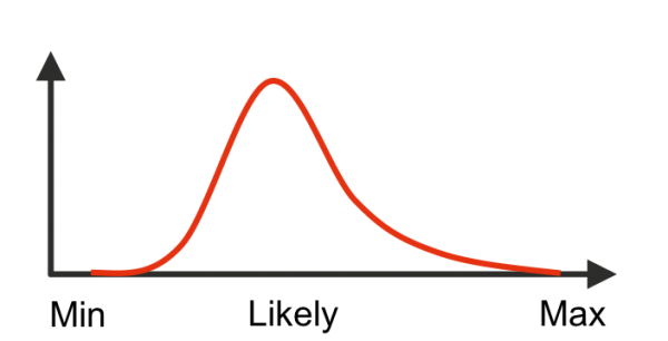
The quotations and other estimates provide an indication of the possible range of actual costs for each item. This range is used to define a probability density distribution for each item, illustrated in Figure 1, in a model built in Excel using the @Risk add-in.
Figure 1: Item cost distribution
The uncertainty in the total cost is evaluated by sampling the item distributions at random and calculating the total cost many thousands of times, a process known as Monte Carlo simulation. Two major outputs are taken from the model:
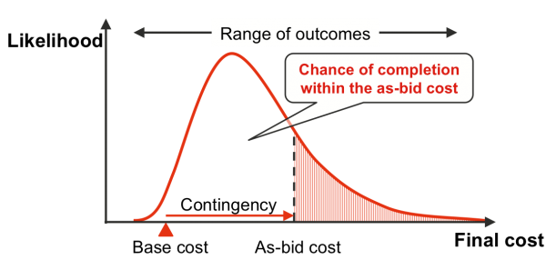
- The distribution of total costs, from which the business chooses a value for the as-bid cost based on the amount of risk that is felt to be appropriate, illustrated in Figure 2
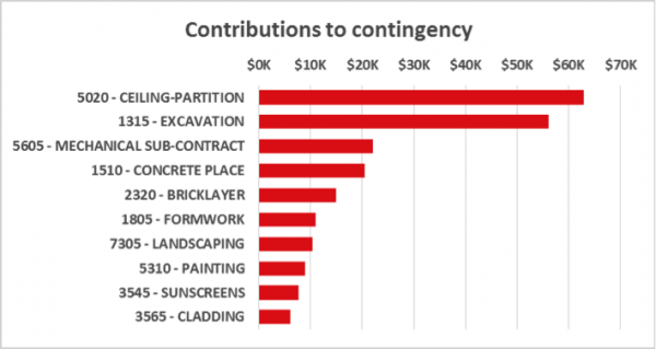
- A summary of the contribution that each item makes to the contingency, which is the gap between the base cost and the as-bid cost, illustrated in Figure 3.
Figure 2: Total cost distribution
Figure 3: Contribution of cost items to contingency
The total cost distribution is used to choose the cost on which the business will base the tendered price. Understanding how far this cost might vary either side of the base cost estimate allows an informed view of how to balance the desire to win against the need to return an acceptable commercial margin. An understanding of the market and experience in the sector are fundamental to the decision. The model provides a tangible framework against which to either confirm the judgements of senior managers or identify areas that should be examined further.
The assessment of how much each of the individual items contributes to the contingency indicates which items have the greatest potential to drive up the cost. This forms the basis of a discussion about where the estimate might be refined and where uncertainty could be reduced, a conversation that can generate useful insights into how to improve a bid.
Project cash flow
Cash flow management during implementation is critical to success in the construction industry. Understanding the cost of a project is an essential first step but not sufficient in its own right.
Technically, there could be a direct link between the cost model and a cash flow risk model but this level of formality is not necessary. The relationship between base costs, cost uncertainty, market price and margin are intimately understood by the business and embodied in an assessment of gross margin uncertainty that is used in the cash flow model.
The cash flow risk model focuses on three dominant drivers:
- Phasing of the cost cash flow during implementation, when costs will be incurred and suppliers’ or subcontractors’ invoices will be paid
- Phasing of the billing cash flow during implementation, when payments will be received from the client
- The margin that the job will yield, a synthesis of the initial cost, the contract price and changes that could arise during implementation.
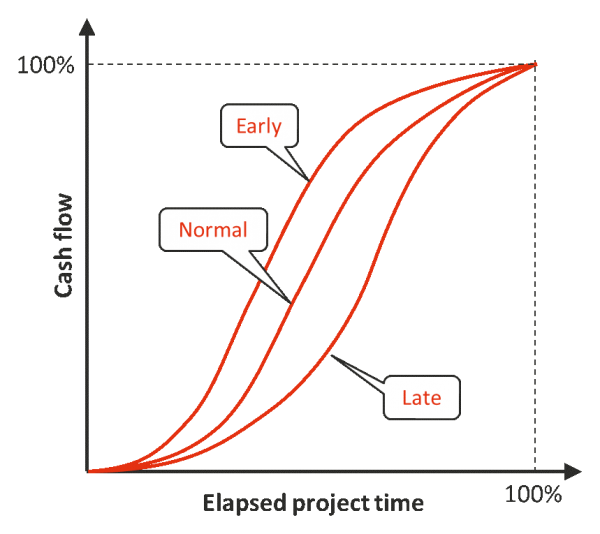
Figure 4 illustrates cash flow timing, showing early, normal and late scenarios for net cash flows across the implementation period. The three S-curves are set by the company’s management team, based on their experience with projects of the kind being considered; this approach is followed for both cost and billing cash flows, so there are three scenarios (early, normal and late) for each.
Figure 4: Cash flow timing
The steps described below are used to examine the effects of uncertainty in a systematic way.
- Establish the nine overall scenarios that correspond to the combinations of early, normal and late outcomes for the cost and billing cash flows.
- Use the company’s existing business systems to calculate the net present value (NPV) for each of the nine combinations, using the as-bid margin determined by senior managers.
- Allow the timing of the cost and billing cash flows to vary uniformly between early and late for each one, and interpolate linearly between the early and late NPVs to calculate the NPV for each intermediate timing scenario. This is the NPV as it would be at the as-bid margin.
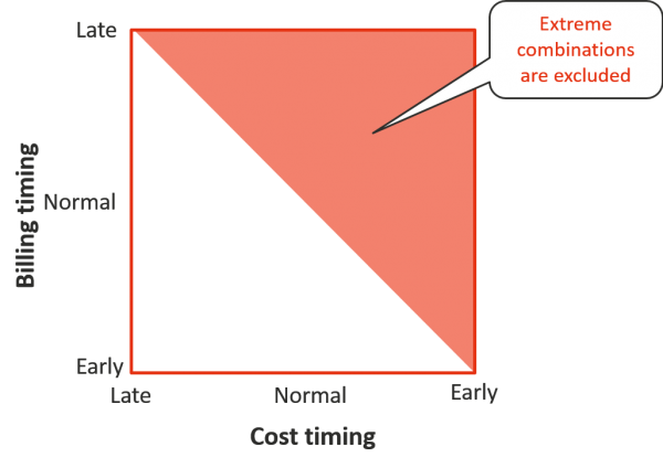
- Exclude the extreme combination of late billings and early costs because it is considered unrealistic, as the control systems of the business are able to reliably prevent this combination from arising. During the simulation, outcomes that result in a combination of cost and billing timings that fall in the shaded region of Figure 5 are removed from the output.
- Overlay margin uncertainty on the intermediate NPV by sampling the margin distribution and applying its variation from the as-bid value. Margin uncertainty is described in terms of a distribution based on maximum, as-bid (most likely) and minimum values.
Figure 5: Avoiding extreme cash flows
As well as demonstrating the range of NPVs that a project might yield, the analysis is used to derive two important pieces of information:
- A ‘safe’ NPV that the business can reasonably rely on from the project, a value lower than the as-bid NPV, see Figure 6
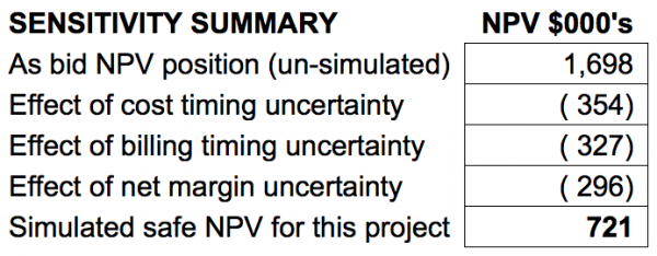
- The proportion of the gap between the as-bid and safe level that can be attributed to the effects of uncertainty in cost timing, billing timing and margin, see Figure 7.
The safe NPV level in Figure 6 provides a risk-averse measure of whether the project is worth taking. The allocation of the shortfall from the as-bid case between the three drivers in Figure 7 offers an indication of where to apply management effort to deliver the as-bid potential of the project.
Figure 6: NPV risk
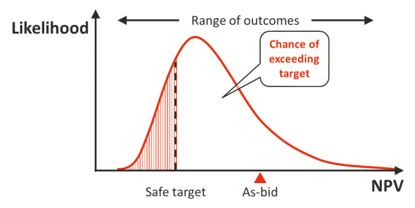
Figure 7: Impact of drivers on NPV
Conclusion
The models used here are not complicated. They are very carefully tailored to work with the financial systems and decision-making processes of the Buildcorp business. They have been pared down to the bare minimum required to be useful for the business.
Several major benefits flow from the use of straightforward tools such as this to support commercial decision-making.
- The numerical outcomes they generate provide a basis for testing commercial judgements and ensuring that inadvertent biases do not unduly influence tendering decisions.
- The process of providing the inputs to the models and discussing the outputs they generate stimulates valuable exchanges within the business about the quality of the inputs and where a bid might be improved before commitments are made.
- The models indicate which aspects of a project will require close attention during implementation to maximise the chances of achieving a high NPV.
A key lesson from this case is that quantitative models do not need to be large, complicated or particularly detailed to make a significant positive contribution to important commercial decisions. They must represent what might happen in the operation of the business in terms that senior managers understand. This can be achieved by carefully tailoring general modelling principles to a particular requirement, so as to preserve the integrity of the analysis while providing a close match to the way the end users think about their work.
If models are simple and realistic, managers can use them to test what their intuition and experience tells them. Quantitative models can never replace human decision making, but if they are constructed carefully they can provide valuable support and insights to help managers add value to their businesses.
- Client:
- Buildcorp
- Date:
- 8 September 2015
- Sector:
- Property
- Services included:
- Project risk management
- Quantitative modelling
- Cost uncertainty
- Contract support