Summary

This case study examines a quantitative risk analysis of the capital costs of a high-voltage power enhancement project. It illustrates the value of integrating quantitative analysis into project workflows, and how the outcomes from the analysis can assist in allocating contingencies to cost items for project cost control. It also demonstrates that the assumptions about the shapes of the distributions used in quantitative analyses may not always have a significant effect on decisions made based on the outputs of the analysis.

Background

The project

A new 330 kV double-circuit transmission line and associated substations were proposed for a regional area. The purpose of the project was to:

• Provide power to existing and proposed energy users in the region, including industrial and mining customers
• Support the installation of new sources of sustainable power generation, including wind farms.

The existing 132 kV transmission lines servicing the area did not have sufficient capacity to meet the increasing needs of the region, so significant network enhancements were required. Construction of the entire line, some 400 km, was scheduled for completion in the next spring, to meet the forecast increase in demand for electricity over the summer.

The new line would replace an existing 132 kV line on wooden poles with the new 330 kV line on steel lattice towers. In one section of the route, a 132 kV line on steel lattice towers would remain in service, parallel to the new 330 kV line. Existing rights of way would be used.

One new substation would be required, and multiple tie-ins and protection changes would be needed at several existing substations.

Project planning and construction would be complicated by the need to dismantle the 132 kV line in stages, to ensure continuity of supply to customers and to integrate the new transmission assets with the existing network.

Risk management requirement

A qualitative risk assessment had been completed for the project. The new requirement was for a quantitative analysis of the capital costs for the project. This was to:

• Investigate and model the residual uncertainties in the cost estimate
• Produce a distribution curve of the range of realistically likely cost outcomes as an input to the development of an agreed project contingency.

The work described in this case study was conducted for the construction alliance that would build the new transmission lines and substations.

Quantitative analysis

Overview

Every project estimate must consider uncertain values and uncertain events. Most items that make up a project’s aggregate costs are uncertain, whether because the complexity and scale of the work has not been specified exactly in advance or because rates cannot be tied down until contracts are let. There may be uncertainty about construction methods and the sequencing of work that will affect costs that cannot be settled until more detailed planning has been completed. Some projects also include uncertain events with the potential to add lump sums to the costs; usually these are unlikely events that cannot be addressed by contract terms, hedging or insurance, but they might also involve interactions with neighbouring property owners, regulators and other stakeholders.

To assess the uncertainties in the cost estimate in this case, the total cost was disaggregated into related parts with common drivers of uncertainty. The uncertainty in each part was described and then the components were combined to form a view of overall uncertainty.

The analysis model was an Excel spreadsheet. In the model, single-value inputs in the spreadsheet corresponding to uncertain items were replaced with distributions of those inputs. Then, the add-in simulation tool @RISK was used to generate a distribution of the overall variation in the capital cost estimate associated with the identified uncertainties. Figure 1 illustrates the process.

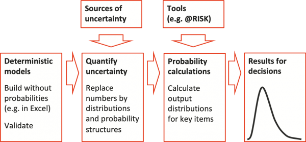
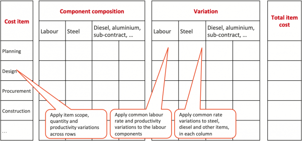
Table 1 provides an overview of the way the cost estimate was disaggregated:

• Individual items were identified (in the left-hand column); variations in quantities, such as variations associated with changes in scope or design detail, were assessed for these items
• Cost components of each part of the estimate were identified (along the top); variations in unit rates and productivities were assessed for these components, although in most cases labour productivities were closely linked to the cost item and nature of the work involved
• The total variation for an individual cost element was calculated as a quantity variation (from the item on the left) multiplied by rate and productivity variations as appropriate (from the component along the top).

This approach allowed many of the cost drivers that are common to two or more items to be accounted for. These common drivers, which cause correlation between the variations in costs, are therefore included directly in the model structure using simple functional relationships. This is both clearer and more realistic than the use of poorly defined correlation factors, especially when quantity and rate drivers overlap.

Cost estimate uncertainty

A cost risk model was developed. This included:

• The main cost items in each remaining phase of the project: planning, procurement and construction
• An estimate of the percentage of the item cost attributable to each main component.

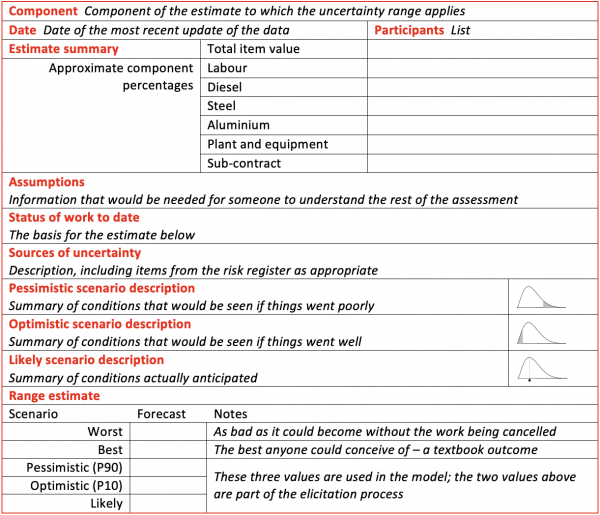
We conducted workshops with the project team and its advisors to investigate and quantify uncertainties in the cost drivers for the estimate. We used a template like the one in Table 2 to capture the data. Templates of this form were also used to estimate the most important uncertainties in the rates for the components, such as hourly labour rates, steel price per tonne and so on. We often use templates like this; this one has been tailored for the project, to record the component percentages for the cost items.

Some uncertainties, such as foreign exchange variations, were excluded from the analysis as they were attributable to the project owner and the risk associated with them would not be managed through the contingency. Some uncertainties were allocated default variations as they related to very low-value items.

The data templates were populated in an initial workshop, reviewed by the project team over the following days, and updated more formally in workshops over succeeding weeks as work progressed and the estimate was refined. The project risk register was also reviewed, to ensure that all material risks had been included in the discussion and analysis.

Distribution assumptions

For each cost driver, uncertainty was assessed in the workshops as a potential variation range defined in terms of a three-point estimate. For each range an optimistic, likely and pessimistic view of the variation from the base estimate was used to define a distribution in the cost risk model.

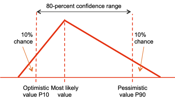
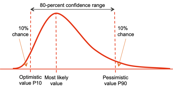
Each uncertain cost driver in the model was represented by a triangular distribution that spreads beyond the optimistic and pessimistic values (Figure 2). The optimistic and pessimistic values defined an 80-percent confidence range, with a 10-percent chance of improving on the optimistic assessment and a 10-percent change of exceeding the pessimistic assessment.

To test the implications of having assumed a triangular distribution shape, we developed another cost risk model with an identical structure and range assessments but in which the optimistic, likely and pessimistic variations from the base estimate defined a Pert distribution like that in Figure 3 instead of a triangular distribution. This allowed us to compare the results of the analysis based on one distribution shape with the results based on the other shape. (The Pert distribution is a variant of the Beta distribution that is often used in project risk analyses.)

Quantitative outcomes from the model

Each cost risk model was developed, using the information from the quantitative risk analysis workshop, and evaluated over a large number of iterations in a Monte Carlo simulation. The range of outcomes and the risk of exceeding values within that range is shown in a distribution of possible contingency requirements (Figure 4), rescaled to preserve confidentiality. The curves show the chance of the required contingency exceeding any specified value on the horizontal axis – the greater the contingency, the lower the chance that it will be exceeded. The solid and dashed lines in Figure 4 show the distributions of contingency using the triangular and Pert assumptions about the shapes of the distributions of variability based on the three-point estimates from the workshops.

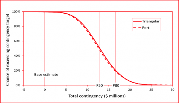
Our client was risk-averse, and intended to set the capital cost contingency at the P80; in other words, our client would tolerate only a 20-percent chance of requiring funds over and above the base estimate plus the contingency. Costs exceeding the funding allocated for the base cost plus the contingency would reduce the company’s profit margin on the project below what was estimated.

As Figure 4 shows clearly, the assumption about the distribution shape makes no material difference to the decision about the total contingency allowance at the P80 confidence level, which was just under $17 million in each case.

Contingency allocation

Our client asked us about most appropriate allocation of the agreed contingency to cost items. The red bars in Figure 5 show the nine largest allocations, covering 90% of the total contingency, calculated on the basis of equal risk. The bars all correspond to item contingencies having the same chance of occurrence for each item, in this case about P65, while adding up to a total contingency equal to the overall P80 value. (The fact that the sum of the P65 values of the cost items is equal to the P80 value of the sum of the cost items reflects the portfolio effect when distributions are added to one another.)

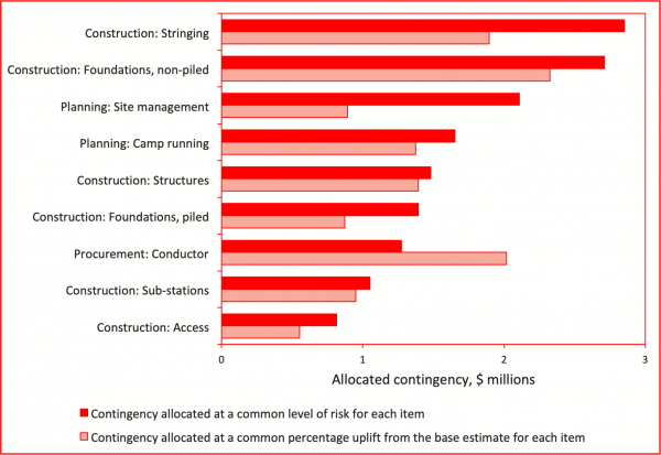
Note that this was only a theoretical exercise, and that the allocation of corporate and project contingency allowances to cost items for management and control purposes may be made on a different basis. A frequently used approach is to apportion contingency to cost items at the same percentage of the item cost, shown in the pale bars in Figure 5. Comparing the two approaches supports common-sense interpretations of project uncertainty; for example:

• Stringing the conductor in the construction phase is more risky than a common percentage uplift contingency might suggest, because stringing usually involves helicopter operations that are highly weather-dependent
• Procuring the conductor, a high cost item in the base estimate, is relatively low risk, in this case because fluctuations in the price of aluminium had been hedged effectively by transferring a large proportion of the market risk to the project owner.

The project team found that Figure 5 provided valuable insights for project cost control and allocation of budgets to managers in different parts of the project. The allocation of budgets and establishment of management targets is a management decision, informed by but not determined by the modelling exercise.

Lessons

'Continuous’ review of uncertainty

The quantitative analysis described here involved an initial workshop, followed by regular reviews and further workshops as work progressed and uncertainties changed. The information about the cost estimate, project risks and their implications for the capital cost contingency, embodied in data templates like Table 2, was always up-to-date, and hence it was a useful resource for the project manager and the project team beyond its use in the analysis.

We commonly find that integrating quantitative analysis closely into the project workflow has substantial advantages:

• It ensures that uncertainty is always front-of-mind for the project team, helping them to direct their efforts to reducing risk and increasing their confidence that the project will achieve its objectives
• Senior decision makers always have available a credible estimate and a credible assessment of the contingency associated with it, based on the level of confidence they require that the funding will be sufficient to complete the project.

Contingency allocation

As the project moves towards the construction phase, graphs like Figure 5 provide insights for the project manager into how contingency might best be allocated. The risk-based allocation illustrated in the red bars in Figure 5 has much more appeal than the pro-rata approach based on a common percentage of item cost illustrated in the pale bars; it allocates contingency based on both the magnitude of the base cost and the amount of uncertainty affecting it. The amount allocated to items with more uncertainty is a larger percentage of their base estimates than the amount allocated to less uncertain items is of their base estimates.

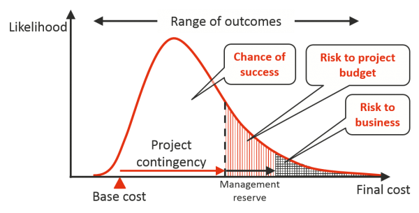
Many contracting companies have policies and standards that deal with contingency allocation and contingency management. Figure 5 shows the allocation of contingency calculated at the P80 level; in practice, a company may only allocate a portion of this, perhaps the contingency calculated at the P50 level or the mean forecast total cost, with the balance held for subsequent allocation at the discretion of the project manager, as illustrated in Figure 6. Graphs like Figure 5 can be adjusted to represent the chosen contingency setting policy as required.

Assumptions about distribution shapes

Figure 4 showed the contingency calculation with two different assumptions about the shape of the underlying distributions representing uncertainty, based on the same three-point estimates of the level of variation.

The Pert distribution in Figure 3 is used when there is a high degree of confidence in the most likely value; the distribution is more concentrated around the most likely value than the triangular distribution in Figure 2. For example, when calculating the mean for a triangular distribution, the three points in the estimate are given equal weights, but when calculating the mean for a Pert distribution the most likely value is given four times the weight of the others. This implies the Pert distribution based on the same three-point estimate is generally narrower and more ‘peaked’, or less risky overall. The triangular distribution can be considered a conservative option as it gives more weight to outcomes in the tails of the distribution than the Pert.

In practice, as illustrated in Figure 4, this distribution shape assumption makes very little difference to the outcomes of the analysis or decisions based on the analysis. With the wide range of uncertainties involved in a typical project, in practice the differences between the assumptions are not material. This is a conclusion that is common to many quantitative project risk analyses with which we have been involved.

Our conclusions are that:

• It may be worth testing the distribution shape assumption, even though it may not be expected to make much difference to the decisions that must be made
• It may not be worth trying to be too sophisticated with individual distribution shapes, despite the apparent ‘special’ characteristics of particular sources of uncertainty
• Nevertheless, testing different distribution shapes may be important for acceptance of the quantitative outcomes, as this may build confidence in the modelling and give the project team a degree of ‘ownership’ of the outcomes.