Enhancing HV power distribution
Summary
A joint venture company was developing a new mine in a remote area. The mine and processing plant would require far more power than could be supplied through the existing high voltage (HV) transmission network in the region.
The enhancement of the regional HV network was to be delivered as a turnkey project. We undertook a quantitative risk analysis of the capital cost of the project on behalf of the power engineering contractor.
The objective of the analysis was to investigate and model the residual uncertainties in the cost estimate for the transmission line enhancement. We developed a model of the range of realistically likely direct cost outcomes as an input to the assessment of an agreed project contingency.
Background
It was planned to build a 330kV infrastructure connection from the existing HV transmission system, to provide a power supply to the new mine site that would be secure and economical in the long-term. The new mine was estimated to require nearly 100MW of power in its first phase, with an additional 150MW as Phase 2 came on stream shortly afterwards.
The power infrastructure connection was divided into 5 sections, summarised in Figure 1 and Table 1. Not all of the components were in the project scope.
Figure 1: Outline of the transmission connection
|
Section |
Components |
|---|---|
|
1 |
Existing 330kV double-circuit transmission line |
|
2 |
New substation and tie-ins, replacing existing substation |
|
3 |
New 330kV double circuit transmission line, replacing existing 132kV line |
|
4 |
New tie-in for existing 132kV transmission line |
|
5 |
New 330kV single circuit transmission line to the mine site off-take point, with a new 330/33kV substation |
Approach
We conducted a workshop to investigate and model the uncertainties in the cost estimate for the transmission line, focusing on the components noted in Table 1. Workshop outputs were used to develop a quantitative model and a distribution curve of the range of realistically likely direct cost outcomes, to form an input to the development of an agreed project contingency. They were also used to develop an estimate of the schedule variation attributable to uncertainty associated with the foundations for the transmission towers.
Participants in the workshop included estimators, power engineers, procurement and contract specialists as well as operations managers.
Workshop outcomes and the base cost estimate were reviewed and refined later by members of the project team.
Quantitative risk analysis
Approach to the analysis
Most items that make up a project’s aggregate costs are uncertain, whether because the complexity and scale of the work has not been specified exactly in advance or because only quoted rates have been obtained from the market. Some projects also include uncertain events with the potential to add lump sums to the costs; these are often unlikely events that cannot be addressed by contract terms, hedging or insurance.
To assess the uncertainties in the project’s cost estimate, the total cost was broken into parts, the uncertainty in each part was described and then the components were combined to form a view of overall uncertainty.
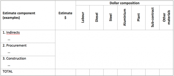
Table 2 provides an overview of the way the cost estimate was disaggregated:
- Individual items were identified (in the left-hand column). Uncertainties in quantities, for example variations associated with changes in scope or design detail, were assessed for these items.
- The cost for each item was broken down according to the cost categories shown across the top of the table. Uncertainties in unit rates were assessed for each category.
- Uncertainties in labour productivities were also assessed for each type of work involved.
- The total uncertainty for a cost element was calculated as a quantity factor (from the item on the left) multiplied by rate and productivity factors as appropriate (from the component along the top), where each factor is one plus the variation from the base case.
Table 2: Estimate summary
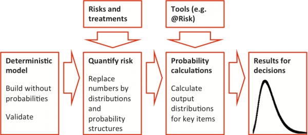
The model was built in an Excel spreadsheet with the @Risk add-in. Single-value inputs to the original estimate where there was uncertainty about the actual value were replaced with distributions of those inputs represented by @Risk input functions. @Risk was then used to generate a distribution of the aggregate variation in the direct cost estimate. Figure 2 illustrates the process.
Figure 2: Including uncertainty in a quantitative model
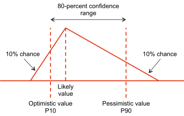
Ranges describing the potential variation in the uncertain quantities, unit rates and productivities were assessed in the workshop as three-point estimates. For each range an optimistic (P10), pessimistic (P90) and likely view of the possible variation from the base estimate was used to define a triangular distribution that spreads beyond the optimistic and pessimistic values far enough to have the same P10 and P90 values (Figure 3).
Figure 3: Triangular distribution interpretation
Detailed cost estimate structure
A cost risk model structure was developed. This was used in the workshop as a guide for capturing the main uncertainties surrounding the cost drivers for the estimate, using structured data tables. Default variation values were used for those parts of the estimate that were not addressed in the workshops (primarily because they were low value items).
Table 3 shows the uncertainties excluded from the estimate, or assigned default values, with comments on the rationale.
|
Item |
Rationale |
|---|---|
|
Access tracks |
Risk taken by the mine owner on schedule of rates |
|
Acid sulphate soil |
Risk taken by the mine owner on schedule of rates |
|
Aluminium price |
Risk taken by the mine owner |
|
Cut-ins |
Not a material cost, not identified separately in the estimate |
|
Foreign exchange |
Risk taken by the mine owner via invoices in USD |
|
Foundations design |
Risk taken by the mine owner on schedule of rates |
|
Import duty |
Rate for aluminium fixed (assuming Bahraini supply of conductor), only volumes can vary; no duty on steel |
|
Labour site allowance |
The mine owner’s labour agreement was assumed to apply, without variation |
|
Other materials rates |
Balance for other materials apart from rebar, concrete and water were set to default variation |
|
Port clearance and inland transport |
Haulage rates were agreed, only volumes could vary |
|
Schedule variation |
Treated separately |
|
Site management and engineering |
Balance after professional staff costs given default variation |
|
Start date variation |
Treated separately |
|
Steel price |
Fixed price quote |
Outcomes from the analysis
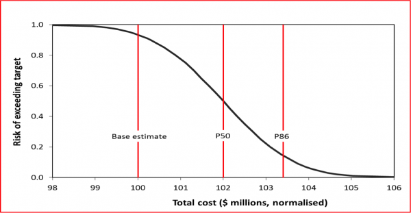
The cost risk model was developed, based on the information from the quantitative risk analysis workshop and subsequent refinement, and evaluated using Monte Carlo simulation. The range of outcomes and the risk of exceeding values within that range are shown in Figure 4 and Table 4. The main curve shows on the vertical axis the risk of the cost to the contractor exceeding any specified value on the horizontal axis. The line labelled P86 is set at the base cost estimate plus the initial contingency, which was set before the quantitative analysis was conducted. This initial value of the contingency had roughly a 14% chance of being exceeded. (The values have been normalised to a base cost of $100 million and do not include the contractor’s commercial margin.)
Figure 4: Cost distribution
|
Percentile |
Value ($ millions) |
Variation from base |
|---|---|---|
|
P7 (Base) |
100.0 |
0.0 |
|
P50 |
102.0 |
2.0 |
|
P60 |
102.3 |
2.3 |
|
P70 |
102.7 |
2.7 |
|
P80 |
103.1 |
3.1 |
|
P86 (Base + initial contingency) |
103.4 |
3.4 |
|
P90 |
103.7 |
3.7 |
Discussions in the workshop, and the corresponding model results, indicated that the mine owner had taken a significant amount of the project risk. Nevertheless, the contractor had some residual exposure:
- The base cost estimate was relatively optimistic, with only a 7% chance of achievement, based on the uncertainties and assumptions discussed in the workshop.
- The initial contingency provided an 86% chance of achievement. In other words, there was a 14% chance of the cost over-running the base estimate plus the initial contingency.
These conclusions depended on the assumptions about the allocation of risk through commercial mechanisms being valid. In particular, if contract negotiations with suppliers were extended for more than 45 days, when many of the quote validity periods expired, these results might not be a good indication of the risk to the contractor.
Lessons
A simple model of the capital cost was sufficiently detailed to inform the commercial decisions that the engineering contractor had to make. It did this in several ways:
- The process of identifying the main drivers of uncertainty and structuring the cost estimate to make their effects explicit was a useful way of highlighting the matters that had to be either resolved before a contract was signed or covered appropriately by contract terms and conditions. By the time the final model was reviewed, the mine owner had accepted many of the most important uncertainties (as indicated in Table 3), thus reducing the risk to the contractor.
- The model itself provided a quantitative guide for the commercial negotiations, as well as a structure within which the effects of further risk allocation decisions (in the form of contract terms negotiated between the contractor and the mine owner) could be evaluated.
- Client:
- Power engineering contractor
- Sector:
- Mining and minerals processing
- Energy
- Services included:
- Quantitative modelling
- Cost uncertainty