Cost and schedule risk analysis for a large resources project
Summary
This extended case study describes a cost and schedule risk analysis for a multi-billion dollar resources project. It illustrates:
- The development of structures for quantitative modelling of cost and schedule, incorporating drivers of uncertainty in quantities, rates and productivities
- How input data for the models can be derived in a workshop environment, to minimise the effects of important estimating biases
- How cost and schedule uncertainty can be integrated in the analysis
- Several forms of sensitivity analysis to support better understanding of the effects of uncertainty and the allocation of contingency amounts across the project.
Background
This case study concerns a multi-billion dollar resources project in a remote location. The project involved the construction, acquisition and development of a mine, mining equipment, ore processing plant, waste and tailings disposal areas, power plant and associated infrastructure, and camp, transport and logistics infrastructure.
The case describes the outcomes from a quantitative risk analysis of cost and schedule components of the project at FEL2 (front-end loading stage 2, often called pre-feasibility, when a preferred project option has been selected for more detailed engineering). The outcomes were to be part of the information package being prepared for approval to proceed to the FEL3 or feasibility stage of the project.
The purpose of this analysis was to examine the uncertainty associated with the current project approach and plan, as well as the associated cost estimate, for the preferred project option from the pre-feasibility study. There may have been alternative execution strategies but they represented strategic choices rather than sources of uncertainty. This was an important basis for the analysis: confusing alternative plans with uncertainty in the current plan would have undermined the purpose of this exercise.
General approach
Analysis overview
The general approach that was adopted for quantitative cost risk modelling is illustrated in Figure 1. It involved:
- Developing an Excel structure, based on the FEL2 capital cost estimate
- Conducting a workshop to elicit information about uncertainty in the cost estimate in the form of distributions and supporting information
- Using the @RISK simulation add-in to calculate the distribution of capital cost, from which a contingency amount can be derived according to the company’s risk appetite.
Figure 1: Outline of the quantitative approach
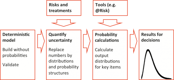
The schedule risk modelling approach was similar, except that the core analysis engine was a tool for schedule modelling, Primavera Risk Analysis (formerly known as Pertmaster), rather than Excel with @RISK.
The outputs of the schedule analysis were exported from Primavera Risk Analysis and used as inputs to the cost risk model to drive duration-dependent costs.
Exclusions from the analysis
The following matters were excluded from the quantitative analysis:
- Sunk costs, including early works
- Variations in plant ramp-up duration
- Escalation
- Foreign exchange impacts
- Finance charges
- Corporate management reserves.
These exclusions do not reflect a lack of interest in the uncertainty associated with these matters. They were addressed elsewhere with personnel who had relevant expertise. The analysis described here was undertaken with engineers, estimators and planners.
The original intent was that sustaining capital be excluded. However, there were many factors applicable to both initial and sustaining capital, so it was decided to include it in the analysis, but to report the outcomes separately.
Some of the initial analyses of rates included market-related factors. Rates were revised after the initial workshops to remove market-related effects for separate consideration as part of the escalation analysis.
For the schedule analysis, only variations after the granting of approval to proceed were included in the schedule distribution used in the cost model, since the main influence of the schedule on costs is its effect on the project’s indirect costs during execution.
Quantitative analysis of cost uncertainty
Model structure
The FEL2 estimate formed the basis for the quantitative analysis. A version of the estimate was exported from the company’s estimating package to Excel, and pivot tables like Figure 2 were used to generate a model structure suitable for quantitative analysis. The aim was for the model to represent a relatively small number of sources of uncertainty that span the bulk of the cost, focussing on the larger WBS items and the major work disciplines (sometimes called commodities).
Figure 2: Estimate structure for analysis
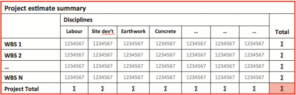
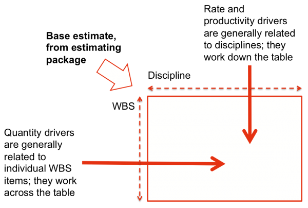
Figure 3 shows an outline of the model structure. This structure allows the drivers of uncertainty in quantities, rates and productivities to be represented separately and applied in a meaningful way to the costs. It is in a form that reduces the amount of correlation between cost items by representing the factors that would lead to correlation as functional relationships, important because failure to account adequately for correlation usually leads to significant errors in the model outputs.
Figure 3: Drivers of uncertainty in the cost estimate
Input data for the analysis
Information about the main drivers of uncertainty was collected in a two-day workshop with members of the project team. They were reviewed on the following day, with a particular focus on ensuring the rates did not contain any market-related variation, as this was to be dealt with as part of escalation, leaving uncertainty about the veracity of quotes and sourcing options to be included in the model. Making realistic assessments of the uncertainty in estimates and forecasts is challenging. There are many ways in which unrealistic assessments can arise.
The method used in these workshops was designed carefully to promote realistic assessments of the uncertainty in costs, either directly or in terms of factors driving the costs. It was based on a deliberate sequence of thinking: first about the background of an assessment, then about what might cause the actual outcome to vary from the forecast and then about the numbers that quantify the uncertainty, which were also gathered in a very specific sequence to limit the effects of anchoring bias.
Figure 4 shows an example of the template used to collect information in the workshops. The data sheets were structured to:
- Capture information about the main assumptions underlying the estimate and the major uncertainties
- Allow a range of scenarios to be developed and documented in outline
- Capture key parameters to allow uncertainty to be quantified and represented as factors in distributional form, while avoiding some of the more obvious biases to which people are prone when they make quantitative estimates of the kind required here.
Figure 4: Data collection template
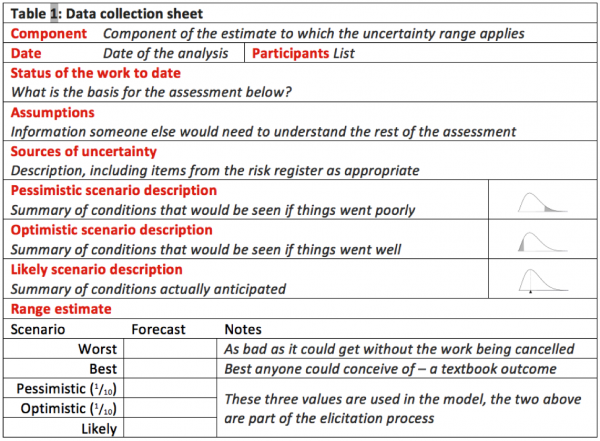
Figure 5 illustrates the sequence in which data was sought, in an attempt to reduce the effects of the anchoring and adjustment bias:
- Numbers are assessed in the order shown, working from the outside of the possible range inwards and from pessimistic to optimistic
- The extreme values are uncomfortable to contemplate; they help break the anchoring effect that otherwise usually leads to unrealistically narrow ranges, but they are not used in the quantitative model
- The pessimistic and optimistic (one in ten, or P10 and P90) values are used in the model as credible poor and good outcomes; values with a one-in-ten chance are within the experience of most estimators and hence are likely to be more reliable for modelling purposes
- The most likely outcome is the value with the highest chance of happening
- The P10, P90 and most likely values define a distribution representing the uncertainty in the factor.
Figure 5: Data collection sequence
For each source of uncertainty, the P10, most likely and P90 values were used to define a triangular distribution. (Empirical evidence suggests that the precise form of the distribution that is assumed in models for projects like this has little practical effect on the model outcomes, at least in terms of the most important decisions they support.)
Calculations in the quantitative model
Each cell in the model contains a formula that multiples the base estimate for that part of the estimate by factors representing the uncertainty in material quantities, unit rates, productivity and the schedule, or a subset of these as appropriate.
= Base × Quantity factor × Rate factor × Productivity factor × Schedule factor
This structure simplifies the analysis:
- Correlation is largely embedded in the structure rather than identified and estimated separately, an alternative approach that is rarely satisfactory
- There are fewer sources of uncertainty to consider
- Effort is focused on the items that are significant in the context of the estimate.
As an indication of the scale of the model and the analysis, there were:
- 21 quantity uncertainties
- 16 rate uncertainties
- 2 productivity uncertainties
- Schedule uncertainty (discussed later).
Quantitative analysis of schedule uncertainty
This schedule analysis was focused on uncertainty associated with the current plan for the project. A fully linked schedule was prepared as the basis of the schedule risk model. It was similar to the Level 1 schedule summary for the project with the high level activities linked logically. This was intended to represent the major blocks of work in sufficient detail to allow the effects of major areas of uncertainty to be represented, while avoiding detail that was not necessary for the analysis.
At this pre-feasibility stage, the analysis did not address ramp-up of the processing plant, the time period between completion of commissioning of the plant and it achieving steady-state production levels. The company recognised there would be value in considering uncertainty in the ramp-up duration later, as it is often a major driver of a resource project’s economic performance.
At this level and for this project, uncertainty in the activities was described directly in terms of their overall durations.
A one-day workshop was conducted with members of the project team, using a workshop process and data sheets like those for the cost analysis.
Integrating the cost and schedule analyses
We did not attempt to create a single, integrated, cost and schedule model for this project. It was not needed at the pre-feasibility stage, and the time and effort required could not be justified.
Instead we built two models that we linked.
- The schedule model was a stand-alone model in Primavera Risk Analysis
- The output from the model was exported as a distribution of variability around the planned start date
- This distribution was inserted in the cost model, and used as a factor to adjust the time-variable costs.
The time-variable costs were all associated with indirect cost items, although not all indirects were time-variable (Table 1).
This approach provided a simple yet effective means of including the most important effects of schedule uncertainty in the cost model. It was fit-for-purpose in this case.
|
Fixed |
Time-variable |
Total |
|
|---|---|---|---|
|
Direct costs |
60% |
- |
60% |
|
Indirect costs |
15% |
25% |
40% |
|
Total |
75% |
25% |
100% |
Outcomes from the analysis
Overall outcomes
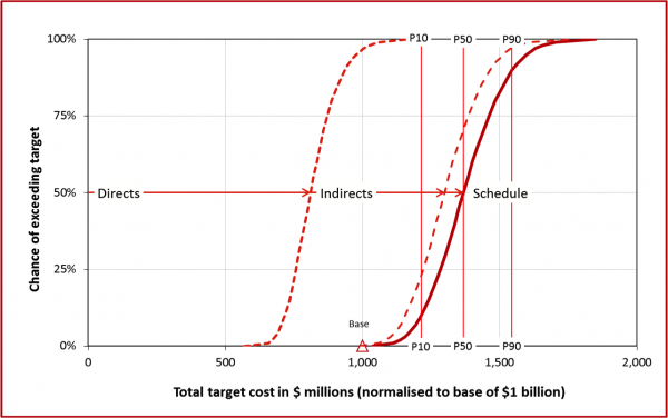
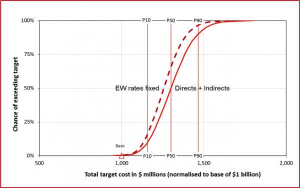
Some of the main outcomes from the analysis are shown in the diagrams that follow. Figure 6 shows the uncertainty in total cost, normalised to a base of $1 billion to ensure client confidentiality, with the contributions of uncertainty in direct and indirect costs and the project schedule. Table 2 summarises the main components of the capital cost contingency, rounded to the nearest $10 million.
Figure 6: Cost distribution
|
Item |
Value ($m) |
Notes |
|---|---|---|
|
Direct cost |
640 |
Base value from estimate |
|
Indirect cost |
360 |
Base value from estimate |
|
Subtotal |
1,000 |
Base estimate |
|
Cost contingency |
300 |
P50 from quantitative cost analysis minus base direct and indirect costs |
|
Schedule contingency |
70 |
P50 schedule cost from quantitative analysis |
|
Project total |
1,370 |
Drivers of cost uncertainty
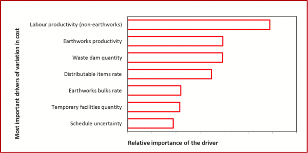
Figure 7 shows the main drivers of cost uncertainty, with an indication of their relative importance – these are what have most influence on the spread of the cost distribution in Figure 6, for example between the P10 and P90 values.
Some of the drivers of uncertainty are discussed further in Table 3. Reducing the uncertainty in these drivers should be an important focus of the next phase of work for the project team. If uncertainty in these items could be reduced then the overall uncertainty in the estimate, and hence in its range of possible values, should reduce.
Figure 7: Drivers of cost uncertainty
|
Item |
Notes |
|---|---|
|
Productivity |
Productivity had an impact on all consumables, construction equipment and labour throughout the estimate |
|
Distributables rate |
Distributables formed a very large component of the total cost, and so uncertainty in the distributables rate was a major driver of uncertainty |
|
Earthworks-related quantities |
Uncertainty in quantities, primarily earthworks, was due largely to uncertainty in the geotechnical conditions, and uncertainty in hydrology to a lesser extent; geotechnical uncertainty was a common driver of quantity variations throughout the estimate |
|
Earthworks bulks rate |
Uncertainty in the earthworks bulks rate had a high upper limit due to uncertainty in the proportion of waste, pre-strip and potentially acid-forming (PAF) material, the quality control over quarried material and quarry development costs; some of these were related to geotechnical uncertainty, as noted above, but other factors were important too |
|
Schedule variability |
Most of the indirect costs (with the exception of temporary facilities) were affected by the schedule; geotechnical and productivity uncertainty were important drivers of schedule variability, both of which have been noted above |
Contributors to contingency
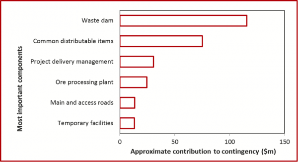
Figure 8 shows the main WBS contributors to the overall cost contingency. For this project the cost contingency was defined as the difference between the base cost and the P50 value from the quantitative analysis.
This contingency was allocated to individual WBS items on the following basis:
- Each individual item contingency was calculated as the difference between the item base value and a Pxx percentile value that was set at a common percentile for all items
- Pxx was varied so that the individual item contingencies summed to the overall project contingency
- In effect this was an ‘iso-risk allocation’ of contingency.
Schedule effects were not included in this calculation.
Figure 8: Contributions to the contingency amount
Earthworks uncertainty
As noted above, uncertainties in earthworks quantities and rates were important drivers of variability in the cost outcome. To provide an indicator of the effect of this uncertainty, we compared:
- The cost estimate including all sources of uncertainty
- The estimate if earthworks quantity and rate uncertainties were eliminated (i.e. set to zero variations).
Figure 9 shows the effect graphically. It allows an estimate to be made of the variability that could be attributed to earthworks uncertainty. Note that schedule uncertainty is not included in either of the distributions in Figure 9, so it is not comparable directly with Figure 6.
Figure 9: Effects of earthworks uncertainty
Lessons
Scale
This was a large, complex, multi-billion-dollar project with a large engineering and management team. The cost estimate, at the pre-feasibility stage, contained over 3,000 items. However, the quantitative risk analysis addressed less than 50 sources of uncertainty.
There are several reasons why this was sufficient for the analysis:
- The estimate was simplified from the 3,000+ items using pivot tables, to allow effort to be focused on the most important parts of the WBS and the major work disciplines
- The sources of uncertainty that were considered, the risk drivers, were linked to the simplified structure of WBS items and work disciplines on which they would have the most influence
- Sources of uncertainty that were similar or that themselves had common drivers were grouped and addressed together.
In our experience, having only a small number of sources of uncertainty is an appropriate approach.
- It reflects the way the uncertainty is understood by the project team, which is in terms of general effects such as a limited level of engineering affecting quantity uncertainties across many work areas or uncertainty about labour availability driving uncertainty about productivity across related activities, making it a natural framework within which the team can express their assessments
- It allows effort to be directed to the most important sources of uncertainty, which can be addressed in detail, without becoming distracted by less important ones
- It makes the quantitative model easier to understand, validate and test
- This in turn allows senior managers to better understand the project itself and the uncertainties that might affect it
- Additional detail can be included, where it is cost-effective to do so, to elaborate and better understand specific sources of uncertainty, as indicated in the analysis of the effects of earthworks uncertainty illustrated in Figure 9.
Structure and correlation
Proper treatment of correlation is critical in quantitative uncertainty models. In most projects the sources of uncertainty are positively correlated, in the sense that if one source of uncertainty is high then related sources will also be high. If these relationships are ignored then the aggregate uncertainty in the total cost will be underestimated, and in some cases by a significant amount.
Estimating correlation between sources of uncertainty directly, most often in the form of correlation coefficients or cupolas, is very difficult for projects.
- It is necessary to examine each pair of sources to see whether they are linked, and there may be many such pairs, N*(N-1)/2 for N drivers (190 pairs for 20 drivers), so it may be a large task
- There is rarely sufficient pertinent historical information to allow statistical analysis of past data, particularly for projects that are large, complex, in ‘difficult’ locations or otherwise having unique features
- People on project teams have great difficulty understanding correlation, let alone estimating it in the form of a coefficient suitable for a quantitative model.
We chose a different approach. By using a simplified estimate structure with a set of drivers of uncertainty (Figure 3), the quantitative model allowed correlation to be embedded within the structure of the model itself. The drivers of uncertainty could be analysed one by one, and there was no need for the project team to think about correlation at all.
For projects like the one in this case, we strongly recommend that quantitative risk models be based on drivers of uncertainty. Fewer sources of uncertainty need to be taken into account, the process is simplified and demands less of the team’s time than it would otherwise, and difficulties associated with estimating correlations are avoided entirely.
Quantification
Care is needed when eliciting numbers for quantitative analysis, because people make errors:
- There are many innate psychological biases, common to most people, that lead to predictable errors of judgement when numbers are estimated for any purpose
- Project leaders and their teams are more confident than they should properly be about the chances of success of ‘their project’, usually as an unconscious over-confidence bias but occasionally (fortunately rarely, in our experience) as a deliberate attempt to influence a decision
- The implications of the assumptions underlying an estimate may not be fully understood when judgements must be made and only limited early engineering has been carried out.
The processes used in this case study were designed to minimise biases where possible.
- The data recording templates (Figure 4) focussed attention initially on assumptions, sources of uncertainty and specific scenarios, thus increasing knowledge and reducing the chance of over-confidence
- The numerical estimates were obtained in a specific sequence (Figure 5) designed to reduce the effects of some of the more common biases, particularly the anchoring and adjustment bias
- Group reviews of the data sheets confirmed the information they contained
- The model itself was straightforward and transparent so that attention to unexpected results could be traced to the inputs that gave rise to them
- Reviews of the model outcomes, including sensitivity analyses, allowed testing of the outcomes to see if they made sense, an indirect indicator of the adequacy of the inputs.
As well as minimising biases, the process also generated a detailed record of the basis for the estimate and the sources of uncertainty associated with it. This will provide the foundation for monitoring and review, and revision of the quantitative model, as further information becomes available through the feasibility stage of the project. Creating this record, embodied in the data tables, allowed a lot of valuable communication and clarification between members of the project team to be achieved quickly.
Integration of cost and schedule estimates
There are several ways of dealing with cost and schedule uncertainty together.
- The effects of cost and schedule uncertainty can be estimated in separate models, and a judgement made about the way in which one affects the other
- The effects of cost and schedule uncertainty can be estimated in separate models, and the schedule variability can be applied to the time-variable costs in the cost model (the approach adopted here)
- A single integrated model can be built, with common drivers of uncertainty for cost and schedule.
The first approach is very simple but not very effective.
The second approach is a simple extension of the first, but it provides a sound basic estimate of the combined effects of cost and schedule on the project. The cost and schedule models can be built using specific tools appropriate for each. The time-variable components of cost must be identified, but that is usually relatively easy to do. The model structure should allow the first-order effects of schedule uncertainty to be isolated, as shown in Figure 6.
The third approach allows for the most detailed representation of the relationship between the schedule and the cost, but it also involves the most effort and complication.
- A tool that allows both cost and schedule uncertainty to be dealt with in one place is needed
- Explicit links between individual WBS items and individual activities in the schedule are often required, and not all of these may be readily apparent or have been addressed in detail during early study work
- The approach to simplifying the cost estimate and the master schedule must be aligned, so the linkages can be achieved effectively
- All of this requires substantially more effort than the second approach, for only a small increase in accuracy.
We chose the second approach for this project. It was sufficient to ensure that schedule uncertainty was incorporated in an appropriate way in the cost analysis, without the very large additional effort required to develop a fully integrated model. The schedule model itself served to highlight the main uncertainties for subsequent attention in the following phase of the project.
Using the model outcomes
The aggregate model outcomes provide an important input to other models that are critical for strategic project decisions.
- The cost and schedule estimates and their uncertainties are major components of models of net present value and associated value metrics used for determining the economic viability of the project, i.e. whether this project is worth doing
- They are also inputs to initial funding and cash flow models used to determine financial feasibility, i.e. whether it will be possible to procure capital to undertake and complete the project, including contingent funds if required.
The detailed model outcomes, including the sensitivity analyses, indicate the main sources of uncertainty in the project cost and schedule. These are likely to be an important focus during the feasibility stage that follows, as the project team’s effort is directed to reducing uncertainty in those areas where it matters most.
- Client:
- International resources company
- Sector:
- Mining and minerals processing
- Services included:
- Quantitative modelling
- Cost uncertainty