Summary

A contractor was preparing a commercial bid to construct a 220/110 kV electricity sub-station. This case describes a quantitative analysis conducted to estimate the effects of potential events on the project cost, as an input to the commercial bid pricing decision.

The case demonstrates how small-scale risk analyses that are fit-for-purpose can be used to support decisions.

Background

A contractor was preparing a commercial bid to construct a 220/110 kV sub-station in a remote site for an electricity supplier. Technically, the project would be relatively straightforward for the contractor, but there were other aspects of participating in the project that would involve risks:

• The bid was expected to be very competitive
• The project was outside the contractor’s usual geographic area of work
• There were some environmental and community issues specific to the site.

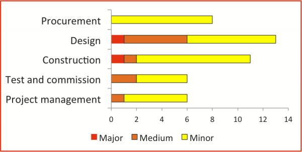
An initial qualitative risk assessment had been undertaken to enhance the project early in its life, in terms of reduced risk exposures for all the parties involved and better project outcomes. It followed the steps in the company’s risk management framework, compatible with ISO 31000 Risk management – Principles and guidelines. This assessment confirmed the relatively low-risk nature of the project, at least in technical terms. There were only two major risks, one related to industrial relations problems associated with acquiring design resources and the other concerned with environmental matters during construction (Figure 1).

A quantitative analysis was conducted subsequently to estimate the effects of potential events on the project cost, as an input to the commercial bid pricing decision. This extended the process to include more detailed analysis and modelling of the effects of risks on those project costs that were not fixed already by contractual arrangements. This case describes the outcomes of the quantitative analysis.

Approach

Overview

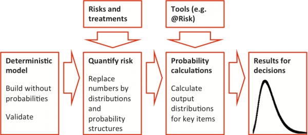
Figure 2 illustrates the approach to quantitative risk analysis that was followed.

• A simple cost model was constructed, based on the cost elements not fixed by the contract
• Scenarios were developed for each uncertain cost element, representing optimistic (P10), pessimistic (P90) and most likely outcomes, and costs were estimated for each scenario
• The three estimates for each element were used to define distributions of costs with the same P10, most likely and P90 values
• Dependence links (correlations) between elements were estimated
• A simulation model with the Excel add-in @RISK was used to derive a distribution of total cost for the project.

Risks and scenarios

Risks are things that might lead to variations in the project cost. They arise from operational matters and they reflect anticipated operating conditions and decisions. In this case, risks included all variations from the project plan that might affect the cost estimate. Both positive and negative variations were taken into account, so opportunities were considered as well as threats.

The focus was on the cost elements that had not been fixed already by contractual arrangements. A high-level estimate structure was appropriate, with 11 elements:

1. Design by contractor
2. Local council approval
3. Busbars 220 kV yard
4. Busbars 110 kV yard
5. Lay and terminate cables
6. 220 kV yard installation
7. 110 kV yard installation
8. Install batteries
9. SCADA equipment and installation
10. Testing and commissioning
11. Project management

The project team estimated the combined effects of all the risks on each cost element, a many to many relationship between risks and cost elements. These were used to develop a quantitative three-point estimate of the potential variation in the cost: P10, most likely and P90 forecasts.

Scenarios were expressed as short descriptions, using a form similar to that in Table 1. A numerical value for the cost of each element was estimated for each scenario, to provide a three-point estimate of the associated cost distribution.

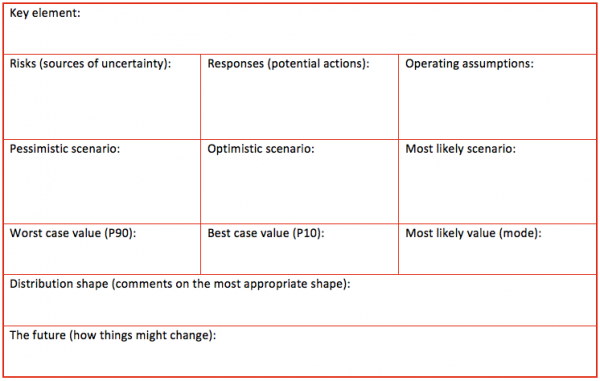
The sequence of scenarios – pessimistic, followed by optimistic, followed by most likely – was used to avoid anchoring and adjustment biases.

• A pessimistic scenario was based on the assumption that everything went badly under the current project plans, an estimate corresponding to there being a 1 in 10 chance of a worse outcome; this scenario represented a reasonable worst case in the sense that it would be as bad as things would be allowed to get in most circumstances
• An optimistic or plausible best case scenario was based on the assumption that everything went reasonably well under the current project plans, an estimate corresponding to there being a 1 in 10 chance of a better outcome
• A most likely scenario was based on the assumption that everything went more or less according to the current project plans.

Outputs from the estimating process included a detailed worksheet for each main cost element, like Table 1, containing a summary of the most significant variations that might affect it and three-point estimates of the potential range of variations.

Cost distribution shapes

For the quantitative analysis, two different assumptions were made about the shape of the underlying cost distributions.

1. An ‘optimistic’ assumption is that the cost follows a Beta distribution (the same distribution used in PERT analysis), which provides a smooth shape with a peak at the most likely value. It is ‘optimistic’ because it is concentrated around the most likely value; in determining the mean of the distribution, the most likely value is given four times the weight of the optimistic and pessimistic values.
2. A ‘risky’ assumption is that the cost follows a triangular distribution, with the apex of the triangle at the most likely value. The triangular shape is ‘risky’ because it generates a wider distribution than the Beta distribution, with a larger standard deviation or spread, and thus more uncertainty.

The quantitative analysis was undertaken using both distribution shape assumptions, to provide an indication of their importance.

Dependence

When combining distributions, it is critical to estimate the dependence relationships or correlations between them. The results from quantitative models may be seriously misleading if they do not incorporate dependence correctly.

Each pair of elements was examined to determine whether there was a relationship or underlying factor that might cause them to vary in the same way. Two sets of dependence links were included in the quantitative model.

1. The costs of the busbars for the 220 kV and 110 kV equipment were linked by the potential variations in the price of aluminium and the labour hours required; complete dependence was assumed
2. There were five elements linked by their mutual dependence on the weather and the contractor’s project management skills; the dependence assumptions are summarised in Table 2.

Combining distributions

The distributions based on the scenario estimates were combined using a simulation approach, taking the dependence assumptions into account. The model was constructed in Excel, and the @RISK add-in was used for the calculations.

Two sets of calculations were performed, one for each of the distribution shape assumptions.

Quantitative outcomes

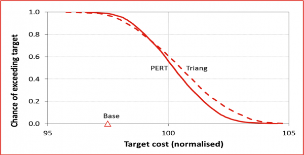
Figure 3 shows the estimated cost distribution for the project cost. There is not a great difference between the results using the PERT and triangular distribution shape assumptions. The triangular assumption is more conservative in the sense that it has a wider spread, hence the flatter cumulative curve in Figure 3, and it was recommended that this be adopted as the basis for the commercial bid. The range of outcomes is relatively narrow, reflecting the low-risk nature of the project and the high proportion of costs that had been fixed contractually.

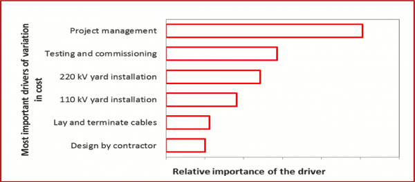
The variation in project management cost is the main source of variation in the overall project cost, shown in Figure 4 for the triangular distribution shape assumption. This is due in large part to the dependence relationships that linked project management closely to other cost elements in the model (Table 2).

Conclusion

Overall, the project was considered to be of low risk. There were two primary reasons for this:

1. The contractor had considerable experience in the design and construction of substations. This substation differed from previous work undertaken by the contractor only in its scale, and steps had been taken to access additional specialist skills to deal with issues relating to the higher voltage ranges involved here.
2. The current project plan involved fixed-price and other sub-contract arrangements for providers of equipment and services that, when implemented, would limit the commercial price risk to the contractor.

Lessons

Scale and scope of the risk analyses

The qualitative risk assessment involved only five key elements (Figure 1). The small number reflected the short time available for the assessment. In practice, the participants had a more detailed project work breakdown structure available for reference during the workshop, and the assessment involved a more extensive consideration of the project than might be apparent from the five elements formally examined.

Similarly, the quantitative analysis only involved a small number of cost elements (11 in this case), as only a high-level analysis was needed. There would have been insufficient time for a complete, detailed analysis, and such an analysis was not deemed necessary for what was viewed as a project with relatively little uncertainty.

The effort devoted to risk assessment, whether qualitative or quantitative, should be tailored to the importance of the decisions that must be made and the uncertainty in the project itself. Both the analyses outlined here generated useful outcomes for the project manager and the commercial manager as they prepared their costed bid, and they were fit for their intended purpose without requiring very much effort from the analyst or the project team.

Quantitative analysis

The distribution shape assumptions represented two quite different interpretations of the scenario estimates. The similarity of the outcomes in Figure 3 gave confidence that the results, and the associated decisions, were relatively stable.

The sensitivity analysis shown in Figure 4 was easy to carry out using the built in capability of the modelling package. It provided information that supported better decisions about how the project might be managed.