An index of the stability of business forecasts
This case study can be downloaded here
Background
Context
Project managers are assessed on their ability to meet targets. They might have performance indicators associated with completion dates and other milestones or with a total cost target. Where a project is being delivered under contract, as opposed to an in-house project delivered by the Owner’s employees, the profit generated by the work will usually be a major focus for the contractor.
In the course of project implementation, progress will be monitored and regular reports will be produced. The forecast completion date, cost or profit will usually be revised in each month’s report. These reports will usually be used to update business forecasts at a level above individual projects.
The work described here concerns the quality of these monthly revisions of the forecast outcome. All else being equal, a business manager will prefer stable forecasts to forecasts that are changed frequently. To date, there have been no metrics in common use that assess directly the stability of the stream of monthly updates to a forecast.
Requirement
A project-based business was concerned about the reliability of project forecasts. There are well-established means for holding project managers to account for the final out turn they achieve but they generally rely on a wrap up of accounts after the work is complete. Our client was concerned not only with the final position, actual profit compared to that anticipated at the start, but also how much confidence could be placed in the revised forecasts issued during execution with each monthly report.
A business generally seeks steady or increasing profits and stable forecasts that allow for efficient cash management. It is difficult to engage managers in a sound discussion about the stability of their forecasts if this is only assessed subjectively.
An objective assessment of stability can provide a structure for a discussion about a project’s performance. Attention can be drawn to consistency, or the lack of it, and the need for early warning of problems. This can be used to tone down unwarranted optimism driving high forecasts that might not be delivered and discourage the provision of deliberate under-estimates offered in the hope of gaining credit for exceeding expectations when the job ends.
The concerns about the stability of forecasts can be illustrated by considering how a business manager would react in a few characteristic scenarios set out in Table 1.
|
Behaviour |
Implications for the business |
|---|---|
|
Initial forecast remains unchanged throughout the project and the final outcome is as it was initially forecast |
Satisfactory |
|
The initial forecast is unchanged throughout the project and the final outcome is better than forecast |
Satisfactory to some extent, but this means that an opportunity to reduce debt or pay additional dividends has been lost |
|
The initial forecast is unchanged throughout the project but the final outcome is worse than forecast |
Unsatisfactory, both because the profit was lower than expected and because this only became apparent at the very end of the project, when there was no further opportunity to remedy the situation or to take it into account in the cash flow management of the business |
|
The initial forecast is varied each month, up and down, and the final outcome is as forecast |
Even though the outcome is as forecast, the uncertainty created by the monthly variations may lead to additional liquid funds being maintained when they could have been used to reduce debt or pay dividends |
|
The initial forecast is varied each month, up and down, and the final outcome is better than forecast |
The uncertainty created by the monthly variations may lead to additional liquidity being maintained when funds could have been used to reduce debt or pay dividends |
|
The initial forecast is varied each month, up and down, and the final outcome is worse than forecast |
In addition to concern about the overall shortfall, the uncertainty created by the monthly variations may lead to additional funds being maintained when they could have been used to reduce debt or pay dividends |
While most people will understand the difference between a steady forecast and one that moves up and down erratically from month to month, a purely subjective assessment can be challenged with assertions of bias. Broadleaf developed a mechanism that introduces a degree of objectivity to the process by producing an index that responds to the pattern of a forecast. This index rises when a forecast is improving or stable and declines when it is falling or unstable.
A simple measure of variation, such as a mean square deviation, was quickly discounted as it has no direct connection to the relationship between cash flow and business performance. It was important to construct the index so that it reflected what mattered to the business rather than just the abstract variation of a quantity in isolation. This was achieved through the approach described in the next section.
Approach
Principles
For these purposes, the way a forecast is perceived as it is updated each month can be summarised in three principles.
- Increasing profit is preferred to maintaining the initial forecast, which is preferred to falling profit.
- Early warning of a change in the forecast is preferred to late warning.
- No change is preferred to a change that is later reversed, whether that change is positive or negative.
The reason for the first rule is obvious. The second rule relates to the ability of the business to manage its cash flows and the flexibility offered to management by early warning of the actual outcome. The third relates to the confidence that management can have in revisions to the forecast during project execution. Calculation
The principle by which the preferences described in the previous section are linked to the business is to regard a forecast as a commitment, by the project to the business, which has value to the business. This value relates to the financial magnitude of the forecast and the length of time for which it is offered.
The value Vk of a forecast at month k during project execution is calculated according the following rules, where F0 is the initial forecast of the final profit, Fi is the forecast issued in month i and 0 < i ≤ k.
An increment is calculated each month and accumulated
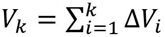
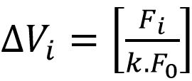
If Fi ≥ Fi-1 then
If Fi < Fi-1 then
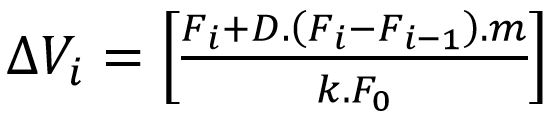
where m is the number of months since the forecast was larger than Fi and D, a value greater than one, is the penalty factor applied to weight falls in the forecast more heavily than rises.
The effect of these rules in some of the scenarios outlined earlier is described in Table 2.
|
Behaviour |
Implications for the business |
|---|---|
|
Initial forecast remains unchanged throughout the project and the final outcome is as forecast |
The monthly increments are all the same (rule 2) and result in an index of 100% in every month. |
|
The initial forecast is unchanged throughout the project and the final outcome is better than forecast |
The final month adds a little to the index in that month so it is a little higher than 100%. The responsible manager may be rewarded for the better than expected outcome but not as much as if it had been foreshadowed earlier. |
|
The initial forecast is raised early in the project and this is delivered |
Raising the forecast increases the contribution made each month (rule 2) and the final outcome is significantly higher than 100%. The responsible manager may be rewarded for the better than expected outcome and also for identifying this early. |
|
The initial forecast is unchanged throughout the project but the final outcome is worse than forecast |
The index of this forecast is 100% in each month up to the end when it is reduced significantly. The reduction is large because it relates to the loss of profit that had been on offer all the time since the project started and because losses are weighted more than gains. The penalty is equal to the amount withdrawn from the forecast weighted by the number of months for which it had been included in the forecast and the penalty factor (rule 3). |
|
The initial forecast is reduced early in the project and the project actually delivers this revised lower level of profit |
Reducing the forecast causes a one off penalty as described in the previous row of this table. Each month’s contribution after that is lower than it would have been but better than the month in which the fall was declared. Steady performance following the fall gradually improves the rating but it remains lower than 100%. The responsible manager may be penalised for the overall reduced profit but less so than if it had not been identified early. |
|
The initial forecast is varied each month, up and down, and the final outcome is as forecast |
The index rises when the forecast rises (rule 2) but declines by a greater amount when it falls (rule 3) so each rise and fall produces a net reduction. The rating at the end of the project is a lot lower than 100%. |
Examples
To illustrate the operation of this index, a series of forecast profiles is shown in the following figures. Each figure is followed by a brief note on its significance. The forecast final profit values are shown as a percentage of the initial forecast and, for convenience, all the examples are based on a twelve-month project duration.
Figure 1: Forecast unchanged throughout
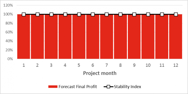
With the forecast being maintained at its initial value and that actually being delivered, the index returns a value of 100% in every month and at the end.
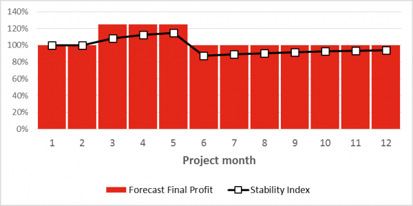
Figure 2: Early declaration of an improved forecast
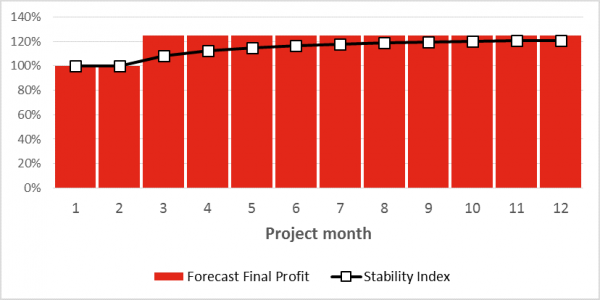
The benefit of an early declaration of an increased forecast that is then sustained is reflected in the rising index.
Figure 3: Late declaration of in improved forecast
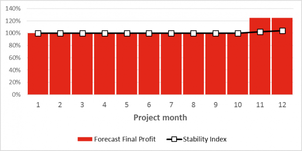
Producing a profit better than initially forecast, at the last minute, has some value but not as much as if it had been visible to the business earlier in the project’s life. Its impact on the index is small.
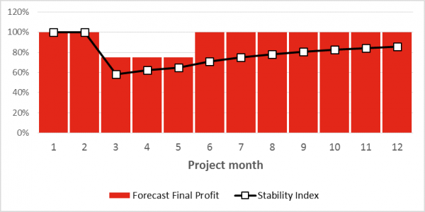
Figure 4: Early declaration of a reduced forecast
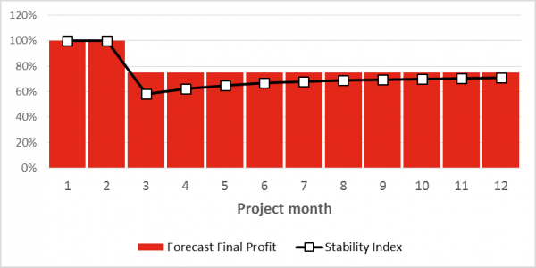
A fall in the forecast of the same amount as the rise shown in Figure 2 causes the index to drop sharply. The steady performance from there on recovers this deficit but does not eliminate it.
Figure 5: Late declaration of a reduced forecast
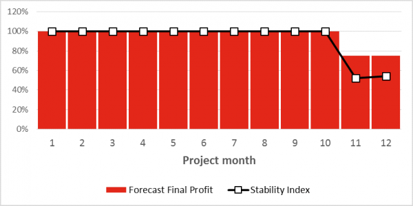
The fall in the forecast here is the same as in the previous example, Figure 4, but because it is declared late in the project the index is penalised more and there is less time to recover. The final rating is worse than with the early declaration.
Figure 6: Forecast improvement that is later reversed
The increase caused by declaring an improved forecast is more than wiped out by reversing it three months later. Although the final profit is as it was initially forecast, the index never recovers to 100%, reflecting the undesirable impact of an unstable prediction.
Figure 7: Forecast reduction that is later reinstated
The impact of the early reduction is overcome to some extent by the later reinstatement of the forecast but the index remains below 100%, again reflecting the undesirable impact of an unstable prediction.
Figure 8: Erratic variation in forecast ending as it began
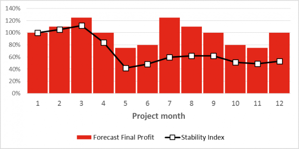
Gains made by offering improved, probably over optimistic, forecasts are more than overcome by later revisions where the forecast is reduced. Although the final profit is as it was initially forecast, the index ends up substantially below 100%, reflecting the undesirable impact of a very unstable prediction.
Conclusions
The stability index described here is simple. It reflects the interest of a business in steady or increasing profits and in stable forecasts that allow for efficient cash management.
As with many models, its value to the business lies in the structure it provides for a discussion about a project’s performance. Using the index month by month, attention can be drawn to the stability of the forecast and the need for early warning of problems. This can be used to tone down any tendency towards bullish overoptimism, which might be reversed later, or over cautious low estimates offered in the hope of gaining credit for exceeding expectations when the job ends.
- Client:
- Building contractor
- Date:
- September 2015
- Sector:
- Property
- Services included:
- Quantitative modelling
- Cost uncertainty
- Contract support