Summary

Broadleaf conducted a review of the implementation program for payroll systems in a group of six related service-delivery networks. Simple Excel structures were used to model the schedule and the uncertainty associated with it. The outcomes provided a structure for activity and manpower planning, as well as a basis for liaison and coordination between the implementation company and the networks.

Background

This case describes a review of the implementation program for payroll systems in a group of related service-delivery networks. The implementation had taken longer than anticipated overall and delays continued to arise in the final stages leading up to going live. Broadleaf conducted the review for the company that was implementing the new systems, with a particular focus on the six networks where implementation had not been completed.

It was particularly important that go-live be handled with care. The effect of a greater-than-usual level of errors in payments to staff or their payslips had the potential to absorb large amounts of effort from both the networks and the implementation company, as well as disturbing the relationship between management and staff.

The review examined the effect of uncertainty in the durations of program tasks on the likely implementation completion dates and resource utilisation. It provided an indication of realistic completion dates and levels of effort for the work.

Analysis

The analysis described was been carried out using a schedule model of the implementation, the structure of which is illustrated in Figure 1 for a typical site. It included the essential components of the implementation company’s project plan for each of the six networks yet to be completed. The model was implemented in Excel using the add-in @RISK, a Monte Carlo simulation package that allows uncertain task durations and uncertain time lags to be represented as distributions and aggregated into a view of the uncertainty in model outputs.

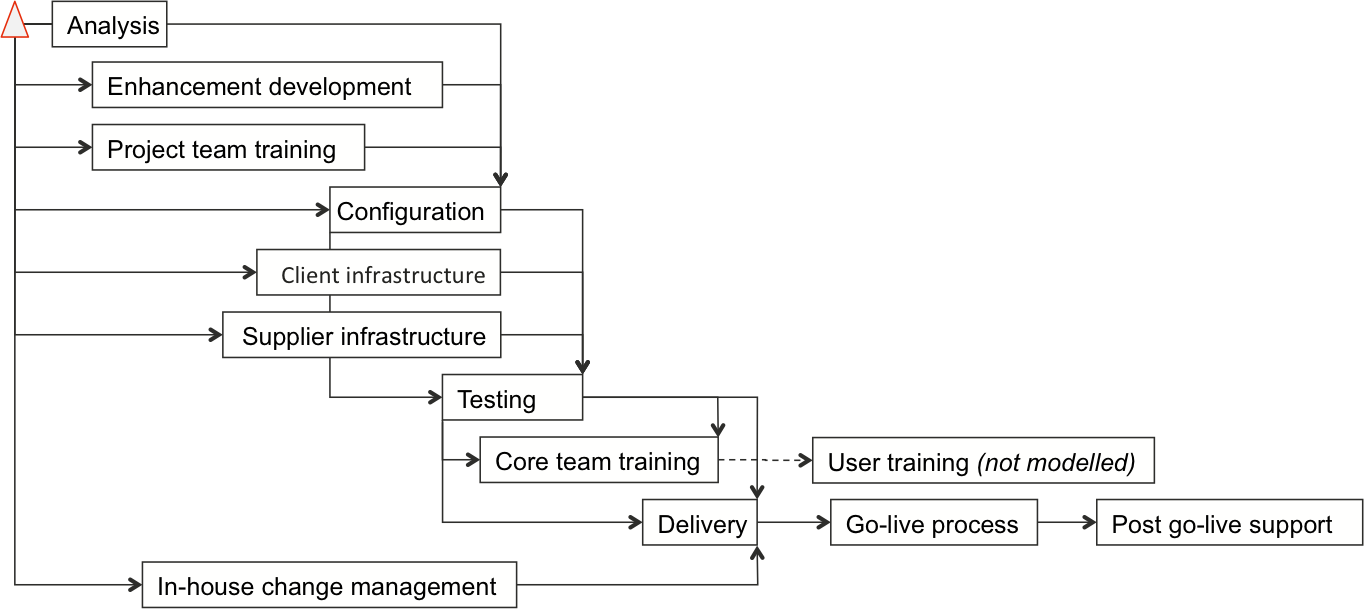
The implementation company’s functional payroll, data conversion and post go-live support resource usage was represented in the analysis. Where activities were resource-constrained across the six sites the affected activities were assumed to run in series. This meant that one site might delay another, depending on how quickly work progressed at each location. Two groups, each of three sites, were dependent on one another in this way through their testing, delivery and go-live activities. The implementation sequences were specified within each group.

In addition, the total effort required from the specialist resources was modelled to estimate the uncertainty in the cost they represented to the program. The effort was modelled as a fixed head count for as long as each task lasted, wherever the implementation company’s functional payroll and data conversion resources were to be used. This meant that the model indicated the effect of the schedule uncertainty on the effort required.

Uncertainty was included in both the implementation company’s tasks and the in-house change management activity that the networks had to complete for a successful go-live. The model represented the net effect of uncertainty arising from both sources.

The Monte Carlo simulation model represented the duration of activities, and lags on links between activities, as distributions.

• For activities that had not yet started, distributions were based on estimates of each component’s minimum, likely and maximum estimated duration
• Activities that were already under way when the analysis began were defined in terms of their earliest, likely and latest end dates
• The model used the actual durations of completed activities as fixed values rather than distributions.

The structure of the schedule dependencies and estimates of optimistic, pessimistic and likely completion dates or durations were provided by senior members of the implementation company’s project team.

The relationships between activities were implemented as formulae in the Excel model, for example to calculate the start of an activity from the latest of the end times of its predecessors. The simulation process generated a random sample of the activity durations that might arise and calculated the go-live dates and resource usage that would result in this case. Go-live dates were constrained to be on a Monday, slipping to the next Monday if they fell on any other day in the simulation.

The model recorded the completion date and effort outputs and then repeated the random sampling process to a total of a thousand iterations. The outputs were summarised as distributions that gave an indication of the realistically likely range of outcomes, the relative likelihood of values in that range and the likelihood of exceeding a target set anywhere within the range.

Model outcomes

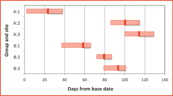
The completion of the go-live activities forecast by the model is summarised in Figure 2. This shows the mean outcome forecast by the model for each site as a thick red line with a bar extending either side showing the range from the 5th to the 95th percentile of the outcomes. Ninety percent of the model outcomes fell within this range.

Figure 2 indicates that, with care, all networks could probably be finished within 130 days of the base date. Site 3 in Group A was the one most likely to test this limit, on the basis of information at the time of the analysis. There was uncertainty of the order of one to two weeks either side of the mean completion dates forecast by the model.

A key feature of each schedule was the date at which a network would have taken its in-house change management to a level at which it felt able to go live (Figure 1). The initial analysis here was conducted for the implementation company, based on the implementation company’s assessment of uncertainty. The delivery networks were not engaged in this analysis, so while the assessment was informed by close involvement with the networks they did not underwrite it.

The amounts of functional payroll, data conversion and post go-live support effort required were also recorded during the simulation. As the model represented activities from the base date onwards, the effort forecasts only related to work from the base date to the end of the implementation.

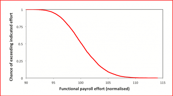
For example, Figure 3 shows the range of functional payroll effort in man-weeks and its distribution, presented in terms of the risk of exceeding any specific value selected within the range of realistically likely outcomes. Values towards the right-hand end of the graph are likely to be achievable with care, but values towards the left-hand end are unlikely to be realistically achievable.

Lessons

Schedule models

The model described here was built entirely in Excel, with the @RISK add-in used for describing the input distributions and the associated calculations, running the simulations and generating the outcome distributions. It was not necessary to use sophisticated schedule risk analysis software.

There were several advantages to this approach:

• The model was seen as uncomplicated by the managers who would need to use its outputs, as they were all familiar with Excel
• The was no black box called ‘quantitative schedule risk analysis’ that managers needed to understand, so there was no inherent scepticism to overcome and explaining the outcomes was relatively straightforward.

Network liaison and coordination

The outcomes from the simulations provided a detailed guide for the implementation company's activities and manpower planning.

They also provided a structure for liaison with the delivery networks and a way of explaining where the networks’ efforts would be essential. In particular, they allowed the single-site view of Figure 1 to be extended to the broader perspective of how activities at each of the sites interacted, and how a delay at one site might have consequences for the implementation at other sites.